Simulation

The virtual lab requires a simulation of the underlying physics occurring during the experiment. In many cases this can be the governing equation for the physics. For example, let's think about the simulation of a simple stress vs strain experiment of an epoxy specimen. Initially, since the epoxy is relatively linear elastic, a reasonable approximation would be to use stress = modulus * strain. And while this approximation would be good for the initial simulation, it would not account for the realistic behavior of necking, and eventual fracture. If we want the virtual lab to be as realistic as possible, then we need the simulation to take into account all of the behavior of the material during this simple test.

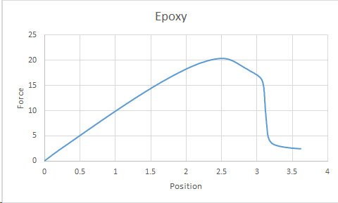
The plot shown here is a extension vs load plot for an epoxy specimen. We would want the simulation to create data that is similar, but not identical. When looking at the plot above, you can identify four distinct regions and we would want our material model (an equation) to capture that behavior.

Assuming you have created a model that captures the material behavior, then the next step is implementing the model to create a reasonable simulation. Every model will have some parameters associated with it. For example for the graph above we would have the initial modulus of the material, the point where the plot becomes non-linear, the slope of the post-failure region, the point where fracture occurs and finally the permanent set associated with the unloaded, failed specimen. In real life all of these regions would be unique to the specific specimen we are testing. So, when implementing the model in the simulation, each of these parameters should be given random values within realistic ranges. Using this approach each time the experiment is run, a realistic but unique result will be obtained.

However, the above model will provide an ideal response that does not include systematic or user initiated error. For this to be a realistic simulation that can be used to replace a real laboratory experience, we need to include systematic and user error. The systematic error is relatively straight forward to include. Experimental apparatus have specifications that provide the sensitivity and error with that particular piece of equipment. Evaluating the systematic error is relatively straight forward and is a topic that is taught in ME 34001. User error includes items like installing the specimen wrong, using the wrong test protocol, reading gauges wrong, etc. Incorporating the user error into the simulation can be done by adding components to the fundamental model or in extreme cases, preventing the simulation from running or damaging the equipment. For example, if the user is running a stress vs strain test and forgets to close the grips on the uniaxial test machine, then the machine will move but the specimen will not be strained and the simulation will not start. Or if the user installs the wrong load cell in the machine, the load cell could break before running the simulation. This behavior would be controlled through scripting.