Algorithm for Quality Measurement of Stereo Image Correlation
Introduction:
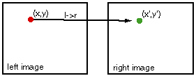
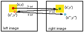
The stereao image correlation software attempts to deliver for every pixel (x,y) in the reference image (left or right) a corresponding pixel coorinate (x',y') in the corresponding pair (right or left). This is depicted in the image below with a mapping from the red point to the green point. This is performed in a parallel algorithm that subdivides the reference image onto different CPUs. The important thing to realize is that the quality of the mapping from left image pixels to right image pixels may not be perfect due to several reasons. Two of the major reasons are: 1) the left eye might see objects that the right eye does not, and vice versa (paralaxe), and 2) the image data might be noisy. The correlation / mapping output delivered by the correlation software may therefore be faulty.
Example Image:
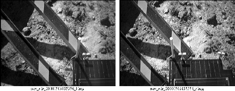
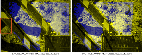
The image below represents an example (image set 1) of a left and right image.
Errors in the Correlation:
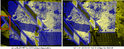
The second row shows the same images with the correlation mask overlayed in blue. The mask indicates that where there is a blue pixel, the correlator thought to have found a corresponding pixel in the other image. A couple of things become rather obvious: the coverage obtained by using the left or the right image as a reference is not the same. Also there is some regions in the left image that appear to be correlated but are not really existing in the right image (see the red rectangle).
Parallel vs. Serial Code Validation:
In the task of the parallelization of the correlation algorithm we certainly want ot measure the quality of the correlation output versus the original serial code output. We originally compared the output of the serial code output to the parallel code output directly and noticed that in large areas we obtain very good agreement , however in other areas we found significant disagreement. Noting that also the serial code might generate erroneous correlation data as indicated above, we needed to develop a better quality assessment algorithm.
Verification of left->right correlation trough right->left correlation:
Following a suggestion by Gary Yagi we decided to assess the quality of the correlation by checking a left->right correlation by a right->left correlation. The basic principle is depicted in the image above. It is based on establishing TWO correlation maps left->right and right->left, therefore doubling the overall workload. The originally desired mapping relates the red point (x,y) to the green point. The corresponding mapping from the green point back to the left will result in the orange pixel (x'',y''). If (x,y) and (x'',y'') are identical we consider this mapping a perfect correlation. The very hard criterion of a perfect match can be relaxed the introduction of an error window (indicated by the yellow square), which accounts for integer interpolation roundoff and a small amount of noise. The influence of this error window size will be explred further below.
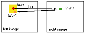
With this right->left and left->right correlation we can establish a quality measure for the for theleft->right correlation data stored at pixel (x,y). Similarly we can establish a a quality measure for the correlation data in every pixel in the right image starting by starting out at a pixel on the right.
There is one more caveat one can consider in this verification scheme which is laid out in the figure below. If one considers a finite window size for the error (yellow square window in figure above) one could encounter a situation depiced in the figure below, where the l->r and r->l verification starting from (x,y) works out fine (red->green->orange), however, the r->l and l->r verification starting from pixel (x',y') does not (green->orange->blue). If such a deviation occurs we should have not accepted the mapping from the green dot to the orange do in the first verification starting at the red dot. We filter such cases out by running the pair of algorithms one more time with the output of the first pass as an input the the new pass through the filter. This way the filtering does bear some sense of self-consistency in it.
Quality Measurement for two image sets:
The image below depicts the number of pixels returned from the correlator as a function of number of CPUs used in the parallel algorithm for image set 1 and 2. There are 4 different quantities depicted here: 1) the raw/uncorrected pixels (largest number), 2) the corrected pixels allowing for 0 pixel deviation during the mapping correction (smallest number), 3) corrected pixels with allowed error of 1 pixel, and 4) allowed error of 2 pixel. The 0 pixel error requirement is very harsh, especially since there can be simple pixel roundoff errors leading to the elimination of a good pixel pair. There is not a large difference in number of corrected pixels allowing for 1 or 2 pixel errors. The graph also shows that hitting the correlator with 10 or 20 maximum seed points does not make much of a difference in the number of returned good pixels, although the number of raw pixels may increase with an increased number of seed points.
Improvements of the Correlation Masks:
The blue colored overlay corresponds to the mask obtained by the serial code after quality check with the algorithm described above (accepted pixel deviation 1). The second row of images corresponds to the parallel algorithm result discussed in the next paragraph.
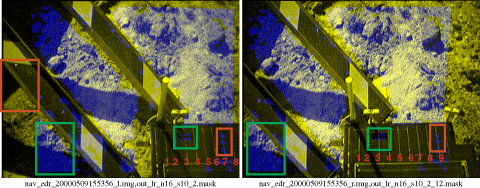
The area that was wrongly correlated in the left image (big red rectangle on the left) has been eliminated by the quality algorithm. The second row corresponds to the results from the parallel code run on 16 CPUs (with 10 maximum seed iterations) after a quality check with the algorithm above (accepted pixel deviation 1). The parallel code does find areas of correlations that the serial code did not explore at all, due to the subdivision of the image (big green rectangle). Some patterns are recognized on the rover (small green rectangle) but other regions are not (small red rectangle).
The second image set:
The figures below show the second image set and the image set with an overlayed correlation mask. No seams are really visible in the correlation mask after generation with 16 CPUs.


Conclusion:
When the correlation data from the serial and the parallel code are compared directly it is found that if both algorithms found correlation data the agreement is identical (0 pixel deviation) for almost all pixels, except for a few tens of pixels that deviate by one pixel. Larger deviations were not found in this example. We conclude that for this image set the correlation algorithm performs just as well as as the original serial algorithm. There are seems stemming from the segmentation of the left image visible in some of the masks, however, if the image correlates well in the serial code, there are no step changes accross the image sections.
Timing Data:
Below the times to calculate the correlation using the "amoeba" algorithm for image sets 1 and 2 are shown as a function of number of CPUs used in the parallel algorithm.

Acknowledgements:
This work was sponsored by the TMOD technology program under the Beowulf Application and Networking Environment (BANE) task.The original VICAR based software is maintained in the Multi-mission Image Processing Laboratory (MIPL). The work was performed in a collaboration between Gerhard Klimeck, Myche McAuley, Tom Cwik, Bob Deen, and Eric DeJong
