This page describes with examples how DEBISim modules can be used to run single baggage simulations as well as create simulated baggage datasets. It also enumerates the various features of the different DEBISim modules and submodules that are used during the simulation operation.
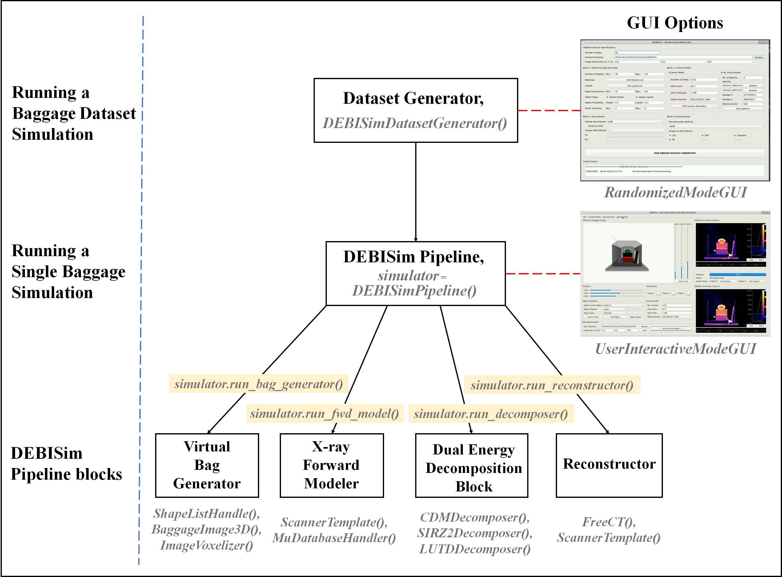
The illustration below shows in a top-down manner the arrangement of
different modules of DEBISim and how they are used for different operations concerning baggage simulation:
From the figure, we can see that the DEBISim simulation pipeline is instantiated by initializing a DEBISimPipeline() class object and the various blocks within the pipeline can be run by calling the appropriate class methods. Simulated baggage datasets are generated by using an instance of DEBISimDatasetGenerator() which loops through randomized iterations of DEBISimPipeline() to create the dataset. Both these operations can be alternately performed by running the GUIs UserInteractiveModeGUI and RandomizedModeGUI respectively. The next sections describe these operations in detail using example scripts.
A simulation for a single virtual bag can be run either by using a class instance of DEBISimPipeline() or by using the User-Interactive GUI, both of which are described ahead. (The example scripts provided below can be found within the /path/to/DEBISim/src/scripts/ directory in the software package):
The DEBISim simulation pipeline is created using an instance of the class DEBISimPipeline() which is initialized by specifying a working directory for simulation, a scanner model generated using ScannerTemplate and the X-ray source specifications. When initialized, the class creates the specified simulation directory and creates the following items within the directory:
| ground_truth/ | This subdirectory holds the ground truth images for the virtual bag. By default, only the label image for the bag, gt_label_image.fits.gz, is saved but other ground truth images (i.e., ground truth Compton, PE, Zeff, CT images) can also be saved while running the simulator. All images are saved as compressed .fits.gz files and can be read using util.read_fits_data() (or any other i/o functions that can process FITS images). |
| projections/ | This subdirectory contains the projection data. The projections are saved as sino_%i.fits.gz, where i stands for: 1, 2 for the DE projections for spectra 1 and 2, 'c' for Compton line integrals and 'pe' for Photoelectric line integrals. |
| images/ | This subdirectory holds the reconstructed single or dual energy CT images generated from the simulation. The reconstructed images are also saved as .fits.gz files. The image files are saved recon_image_%s.fits.gz (where %s - 1,2,… n - for the CT images, 'c' - for compton, 'p' - for PE and 'z' - for effective atomic number.) |
| sl_metadata.pyc | This pickle file contains the Shape List for the simulated bag which describes the different objects spawned within the bag. See ShapeListHandle() for more details. |
The virtual bag for the data simulation can be created manually or in a randomized mode. When in the randomized mode, the simulator calls in the BaggageCreator3D module to create a 3D virtual baggage image with objects randomly selected, placed and oriented as specified by the baggage creator arguments. To create a virtual bag manually, the objects to be spawned in the baggage simulation are specified by a Shape List provided as input. The parameters within the Shape List can be fed in using a User-Interactive GUI or the Shape List can be manually created by specifying the pose and material properties for each object in the image. The following example shows how the DEBISim simulation is run with a step-by-step description of the execution of each of the pipeline blocks.
An example for using DEBISimPipeline in a randomized mode is given below with each of the steps for operation described in detail below the code:
from DEBISimPipeline import *


# ----------------------------------------------------------------------------
# Step 1: Initialize the DEBISimPipeline

# Step 1.1: Specify Scanner Model using the class ScannerTemplate - parameters
# such as pitch, slice thickness can be modified in ScannerTemplate initialization
# The default scanner is Siemens Sensation 32 which is a Spiral CBCT Dual
# Energy Scanner and is specified in the forward_model modules scanner - see
# ScannerTemplate documentation to specify your own scanner configurations.

scanner_mdl = ScannerTemplate(
    scan='spiral',
    recon_dict=siemens_sensation_32.recon_params,
    machine_dict=siemens_sensation_32.machine_geometry
)
scanner_mdl.set_recon_geometry()

# Step 1.2: Specify X-ray Source Model

# The Xray Source Model is specified by a dictionary with the following key-
# value pairs:
# num_spectra - No of X-ray sources/spectra
# kVp - peak kV voltage for the X-ray source(s)
# spectra - file paths for the each of the X-ray spectra. The spectrum files
#           must contain a N x 2 array with the keV values in the first
#           column and normalized photon distribution in the 2nd column. See
#           /path/to/debisim//include/spectra/ for reference.
# dosage - dosage photon count for each of the sources

specdir = './include/spectra/'
xray_source_specs = dict(
    num_spectra=2,
    kVp=140,
    spectra=[os.path.join(specdir, 'imatron_spectrum_140kV.txt'),
             os.path.join(specdir, 'imatron_spectrum_100kV.txt')],
    dosage=[2.2752e6, 8.6648e05]
)

# Step 1.3: Initialize DEBISimPipeline class
simulator =  DEBISimPipeline(
    sim_path='./examples/sim_3d_random/',
    scanner_model=scanner_mdl,
    xray_source_model=xray_source_specs
)

# ----------------------------------------------------------------------------
# Step 2: Run the Virtual Bag Generator block

# Step 2.1: Specify the BaggageCreator3D() Arguments - these
# arguments decide the nature of objects that will be randomly
# spawned in the simulated bags. The arguments contain the list of
# materials that will be assigned to the objects in the bag - the
# material assignment is random and the liquids need to
# be specified separately if liquid filled containers are to be spawned.

mlist    = ['Al', 'pyrex', 'acetal', 'acrylic', 'C', 'Si', 'polyethylene']
lqd_list = ['water', 'H2O2']

bag_creator_dict = dict(
    material_list=mlist,
    liquid_list=lqd_list,
    material_pdf=[1/7.]*7,     # PDF for material selection
    liquid_pdf=[0.5,0.5],     # PDF for liquid selection
    lqd_prob=0.2,      # Probability of spawning a liquid filled container
    sheet_prob=0.3,      # Probability of spawning a deformable sheet
    min_dim=10,       # Range of object dimensions
    max_dim=90,
    number_of_objects=range(20,25),
    spawn_sheets=True,
    spawn_liquids=True,
    sheet_dim_list=range(2, 7),
    custom_objects=None
) # See BaggageCreator3D for details about the input arguments.

# Step 2.1: Call the bag_generator method with mode set to 'randomized'
simulator.run_bag_generator(mode='randomized', bag_creator_dict)
slide_show(simulator.gt_image_3d.cpu().numpy(), vmin=0, vmax=30)

# ----------------------------------------------------------------------------
# Step 3: Run the Forward X-ray Modelling block - creates X-ray projections using
# the specified scanner and source models

simulator.run_fwd_model(
    add_poisson_noise=True, # Add Poisson noise to projections
    add_system_noise=True,  # Add detector system noise
    system_gain=1e2    # system gain
)

# ----------------------------------------------------------------------------
# Step 4: Run the DE Decomposition block

# Step 4.1: Specify arguments for DE decomposition depends on the DE Decomposition
#  module used - see the module API for details

cdm_args = dict(
cdm_solver='gpu', # CPU or GPU operation
cdm_type='cpd', # the bases for decomposition
projector='cpu',
init_val=(1, 1) # initial values for running the optimization algorithm
)

# Step 4.2: Call the decomposer method using CDM Decomposition method

simulator.run_decomposer(
    method='cdm',
    decomposer_args=cdm_args
    )

# ----------------------------------------------------------------------------
# Step 5: Run the Reconstructor block

simulator.run_reconstructor(
    # Determines if images are saved in Hounsfeld or attenuation units
    img_type='HU'
    )
A step-by-step description of the above code is given below for each of the pipeline blocks:
In order to initialize the instance of the DEBISimPipeline, one must first specify (i) a scanner model generated using the ScannerTemplate module, (ii) a Python dictionary specifying the X-ray source model, i.e., the spectrum pdfs, the dosage and the peak tube voltage (see code above) and (iii) a working simulation directory. The four blocks of the simulation pipeline can then be run one-by-one by calling the methods DEBISimPipeline.run_bag_generator(), DEBISimPipeline.run_fwd_model(), DEBISimPipeline.run_decomposer() and DEBISimPipeline.run_reconstructor() respectively.
The virtual bag generator in the DEBISim pipeline is run by calling the DEBISim.run_bag_generator() method. The virtual bag generator can be set to run in a randomized mode by setting mode='randomized' when calling the method. When set to randomized mode, the method must be fed in a dictionary containing the baggage creator arguments that are then fed to the BaggageCreator3D module to create the 3D label image of the randomized virtual bag. These arguments specify the shape, number, frequency and material properties of the baggage contents and are described in detail in the documentation for Virtual Bag Generator. Another option for this block is to run it in a manual mode by setting mode='manual' wherein the bag is generated by reading a shape list (See ShapeListHandle). Both in randomized and manual mode, running the virtual bag generator block creates a 3D label image of a virtual bag which is saved in /ground_truth subdirectory as well as a sl_metadata.pyc file which contains the Shape List.
The forward X-ray modelling block in the DEBISim pipeline can be run by calling the DEBISim.run_fwd_model() method. When called, the method forward-projects the 3D image of the virtual bag into projection space based on the scanner and spectrum model that simulator was initialized with to generate polychromatic CT projection data. If more than one spectra are provided during initialization, the method generates one projection for each individual spectral distribution. The generated polychromatic projections are stored within the /projections subdirectory within the simulation directory. The noise settings for forward modelling can be also be adjusted while calling the method (See code above).
For Dual Energy CT systems, the CT projection pair that is generated from the X-ray modelling block can be processed using a Dual Energy Decomposition algorithm to generate material coefficient line integrals such as for Photoelectric and Compton scattering interactions. Running the DE decomposition block allows to run these algorithms on the projection data created for the virtual bag. The method DEBISimPipeline.run_decomposer() provides us the following options for the DE decomposition which can be selected by setting the type argument for the method:
The line integrals generated by all these methods are saved as FITS files within the /projections subdirectory in the working simulation directory.
[1] Ying, Zhengrong, Ram Naidu, and Carl R. Crawford. "Dual energy computed tomography for explosive detection." Journal of X-ray Science and Technology 14.4 (2006): 235-256.
[2] Azevedo, Stephen G., et al. "System-independent characterization of materials using dual-energy computed tomography." IEEE Transactions on Nuclear Science 63.1 (2016): 341-350.
[3] Patino, Manuel, et al. "Material separation using dual-energy CT: current and emerging applications." Radiographics 36.4 (2016): 1087-1105.
The reconstructor block which is run by calling the DEBISimPipeline.run_reconstructor() reconstructs all the projection data to create 3D CT images for the virtual bag as they would be generated by physically scanning the bag. It also reconstructs the coefficient images from the line integral generated form the DE decomposition block (Compton, PE and Zeff images in case of 'cdm'; Ze, electron density and SMB images in case of 'sirz' and the material basis images in case of 'mbd'). All these images are saved as compressed FITS files in the /images subdirectory within the working directory. The reconstructed images are aligned with the label image in /ground_truth/ subdirectory for annotating the objects within the virtual bag. The image can be reconstructed using the FBP algorithm (recon='fbp') or 3D-SIRT algorithm (recon='sirt') and can be saved in Hounsfield, Modified Hounsfield and CT attenuation units (img_type= {'HU' | 'MHU' | 'LAC'}).
The simulation pipeline can also be run by reading in a previously saved or a user-specified shape list. (See ShapeListHandle or the User-Interactive Mode GUI for information about shape lists.) This simply requires changing the mode in the bag generator block to 'manual' and feeding in the shape list to the simulator.
# -------------------------------------------------------------------------
# Read the pickle file containing the Shape List for ACR phantom -
# Alternatively, a Shape List can be manually created by specifying objects
# within the image, see ShapeListHandle for details.

fpath = './examples/phantom_shape_lists/acr_phantom.pyc'
with open(fpath, 'r') as f:
    data = pickle.load(f)
    f.close()

# ----------------------------------------------------------------------------
# Initialize the X-ray data simulator with the scanner model and source specs
simulator =  DEBISimPipeline(
    sim_path='/home/ubuntu/acr_phantom_simulation/',
    scanner_model=id1,
    xray_source_model=xray_source_specs
)

# ----------------------------------------------------------------------------
# Create the simulation from the Shape List
simulator.run_bag_generator(mode='manual', source=sf_file)
slide_show(simulator.gt_image_3d.cpu().numpy(), vmin=0, vmax=30)
The following are examples of phantoms and randomized bags generated using the DEBISim pipeline:

User-Interactive Baggage Simulation for DEBISim can be performed by using the UserInteractiveModeGUI which allows the user to manually pack a virtual 3D bag using a 3D GUI and run the DEBISim pipeline to create the simulation. This is useful for creating specific test cases and phantoms by manually aligning and manipulating different objects in the 3D baggage image.
The GUI can be used by running the script run_user_interactive_gui.pyc within the src/gui/ directory and the steps for using this GUI are given in the following tutorial.

The section describes how simulated baggage datasets can be generated using the DEBISim pipeline. The two methods for dataset generation (using the DEBISimDatasetGenerator module or the RandomizedModeGUI module) are explained as follows:
The DEBISimDatasetGenerator module is implemented for generation of randomized baggage datasets by iteratively executing the DEBISim pipeline. The operation can be run by calling the DEBISimDatasetGenerator.run_xray_dataset_generator() with specifications for each of the four blocks of the simulation pipeline fed in as input arguments. This is described in detail in the following example:
from DEBISimDatasetGenerator import *

# -------------------------------------------------------------------------
# Step 1: Specify dataset parameters:

bags_to_create = range(5)   # Number of bags to create
sim_dir = '/home/ubuntu/DEBISimDataset_01/' # simulation directory

# -------------------------------------------------------------------------
# Step 2: Specify Scanner Model using ScannerTemplate.py - parameters such as pitch, slice thickness can be modified in ScannerTemplate initialization

scanner_mdl = ScannerTemplate() # Uses default scanner (Siemens Sensation 32)
scanner_mdl.set_recon_geometry()

# -------------------------------------------------------------------------
# Step 3: Specify Xray Source Model

# The X-ray Source Model is specified by a dictionary with the following key-
# value pairs:
# num_spectra - No of X-ray sources/spectra
# kVp - peak kV voltage for the X-ray source(s)
# spectra - file paths for the each of the X-ray spectra. The spectrum files
#           must contain a N x 2 array with the keV values in the first
#           column and normalized photon distribution in the 2nd column. See
#           /include/spectra/ for reference.
# dosage - dosage count for each of the sources

specdir = './include/spectra/'
xray_source_specs = dict(
    num_spectra=2,
    kVp=140,
    spectra=[os.path.join(specdir, 'imatron_spectrum_140kV.txt'),
             os.path.join(specdir, 'imatron_spectrum_100kV.txt')],
    dosage=[2.2752e6, 8.6648e5]
)

# ----------------------------------------------------------------------------
# Step 4: Specify the arguments the BaggageCreator3D() Arguments - these
# arguments decide the nature of objects that can be spawned in the simulated
# bags.
# The list contains the list of materials that will be assigned to the
# objects in the bag - the material assignment is random but liquids need to
# be specified separately if liquid filled containers are to be spawned.

mlist    = ['Al', 'pyrex', 'acetal', 'acrylic', 'C', 'Si', 'polyethylene']
lqd_list = ['water', 'H2O2']

bag_creator_args = dict(
    material_list=mlist,
    liquid_list=lqd_list,
    material_pdf=[1/7.]*7,
    liquid_pdf=[0.5,0.5],
    lqd_prob=0.2,
    sheet_prob=0.3,
    min_dim=10,
    max_dim=90,
    number_of_objects=range(10,15),
    spawn_sheets=True,
    spawn_liquids=True,
    sheet_dim_list=range(2, 7),     # range of sheet thicknesses
    custom_objects=None             # if any custom object shapes to be
                                    # specified
)

# ----------------------------------------------------------------------------
# Step 5: Specify the decomposer and its arguments - if using Dual-/Multi-
#         energy Spectra, a decomposer module can be specified to extract the
#         coefficient integrals. In this case, it is the CDM Dual Energy
#         Decomposer that is specifed, if nothing is specified, the
#         simulation only generates the single energy CT reconstructions.

ntheta = scanner_mdl.machine_geometry['n_views_per_rot'] *scanner_mdl.machine_geometry['n_turns']
ndet   = scanner_mdl.machine_geometry['n_sens_x']

# Specify the parameters for the CDMDecomposer for DE decomposition
cdm_args = dict(
cdm_solver='gpu',
cdm_type='cpd',
projector='cpu',
init_val=(1, 1)
)

# Initialize the CDM Decomposer
sim_specs = dict(
    spctr_h_fname=xray_source_specs['spectra'][0],
    spctr_l_fname=xray_source_specs['spectra'][1],
    photon_count_high=xray_source_specs['dosage'][0],
    photon_count_low=xray_source_specs['dosage'][1],
    nangs=ntheta,
    nbins=ndet,
    projector='cpu'
)

cdm_sim = CDMDecomposer(**sim_specs)

# ----------------------------------------------------------------------------
# Step 6: Run the XrayDatasetGenerator function with the setup arguments
run_xray_dataset_generator(bags_to_create,
                           sim_dir,
                           scanner=scanner_mdl,
                           xray_src_mdl=xray_source_specs,
                           bag_creator_args=bag_creator_args,
                           decomposer=cdm_sim,
                           decomposer_args=cdm_args
                           )
The details on using the DEBISimDatasetGenerator module can be found here:
DEBISim also contains a GUI version of the DEBISimDatasetGenerator module to create randomized CT datasets. The GUI allows specifying the size and characteristics of the dataset as well as the specifications for the constituent blocks for the simulation pipeline - these options are analogous to the arguments fed to DEBISimDatasetGenerator.

The following is an illustration of data samples from a randomized dataset generated using the DEBISimDatasetGenerator module:
