5.3 Belief Propagation (the Sum-Product Algorithm)
As promised, we take a detour through VE on a tree, rather than an arbitrary graph, in order to see how computation re-use can be developed into a message-passing protocol. The key fact about a tree is that there exist elimination orderings that do not create intermediate tables with more than two ways, i.e. the number of ways in the tables parameterizating the original tree.33 3 More generally, for any random variables (not just categorical), the intermediate potentials will be functions of at most two variables. A different way to put this is that, under such elimination orderings, the elimination cliques are just the pairs of neighbors in the tree. Conceptually, this means that we can map the operations of variable elimination onto the original graph; there is no need to construct a second graph.
Variable elimination on a tree.
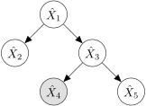
To see this, we begin with an example, computing in the tree in Fig. 5.2a. Using variable elimination and the ordering , we obtain
We could implement this in code as
# compute p(X5|X4=1) with elimination ordering I = {2, 1, 4, 3}
IS_ONE = np.array([1, 0])
omega21 = p_X2givenX1
assert omega21.shape == (2, 2, 1, 1, 1)
m21 = omega21.sum(axis=1, keepdims=True) # = 1
omega13 = p_X1*p_X3givenX1*m21 # = p(X1,X3)
assert omega13.shape == (2, 1, 2, 1, 1)
m13 = omega13.sum(axis=0, keepdims=True) # = p(X3)
deltaX4is1 = IS_ONE.reshape([1, 1, 1, 2, 1])
omega43 = deltaX4is1*p_X4givenX3
assert omega43.shape == (1, 1, 2, 2, 1)
m43 = omega43.sum(axis=3, keepdims=True) # = p(X4=1|X3)
omega35 = p_X5givenX3*m13*m43 # = p(X3,X4=1,X5)
assert omega35.shape == (1, 1, 2, 1, 2)
m35 = omega35.sum(axis=2, keepdims=True) # = p(X4=1,X5)
pX5givenX4is1 = m35/m35.sum()
It is easy to see that, in this example, the intermediate tables omega* all have at most two ways, and the intermediate tables m* all have one way.
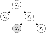
Does this hold generally for VE on trees? Yes, it does, as long as we let the target node be the root of a(n undirected) tree, and then eliminate recursively from leaves to root. (Fig. 5.2b shows the undirected tree for our example, with root at top.) Since the graph is a tree, the maximal clique size is two, and correspondingly each potential function44 4 In a directed tree, these potential functions are conditional probabilities; in an undirected tree, they are arbitrary. references at most55 5 It can reference fewer: the node that was originally the root of the directed tree will have a singleton rather than pairwise potential. two variables. Eliminating a leaf variable therefore yields a one-way66 6 Or zero-way; see previous. table. Broadcast multiplying this table onto the parent’s potential function does not increase its dimensionality (number of ways), since the child’s table, after marginalization, references only the parent’s variable, which is already represented in the parent’s potential function. Once all of the parent’s children have been eliminated in this way, the (former) parent is itself a leaf of the tree, with an updated potential (i.e., table) that makes reference only to (at most) itself and its parent. So the argument generalizes to the whole tree.
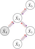
We anticipated above that we would be able to interpret such a run of VE as an operation on the tree. Since every intermediate table m* is computed by marginalizing a child out of a pairwise potential over parent and child, we will think of it as a message passed from child to parent. For the example just discussed, these messages are shown in red in Fig. 5.2b. (We could just as well have used the original tree, Fig. 5.2a, but Fig. 5.2b makes the leaves-to-root order of message passing more perspicuous.)
The computation of any message can be summarized as: once a node has received messages from all of its children—i.e.,77 7 “The neighbors of , excluding .” for all —it can compute
where the functions are the potential functions on the corresponding undirected graph. Note that for directed trees, the singleton potentials are
and the pairwise potentials are
That the message must take the form of Eq. 5.10 follows from the fact, familiar from the Section 5.2, that the sum over will not “push in” any farther than the potentials that reference it. Since, by hypothesis, neither nor its parent have been eliminated yet, the (original) potentials and must be among these. Since the graph is a tree, the only other potentials that can reference must be its children, which by hypothesis have already been eliminated, and therefore have sent their messages .
By variable elimination, the final elimination leaves us with the desired marginal (possibly unnormalized), , with the last (uneliminated) node, and the vector of all the observations. We can also say that it leaves us with whatever has not been eliminated, namely the messages into and (possibly) a singleton potential . (Note that we are not left with any pairwise potentials for any of the children of , because these potentials reference those children, and will therefore have been marginalized into messages.) Therefore the target probability is
For unobserved directed graphs, the proportionality constant will be 1, but for undirected graphs or graphs with observations, the right-hand side will be unnormalized.
Re-using computations.
Mapping variable elimination on a tree onto message passing is neat, but we would like to go further and use this to develop a protocol for computation re-use. To see how to take this last step, consider (as above) computing a different posterior distribution, say, . We will begin again with a run of VE, this time with the elimination ordering :
It should be clear that this series of computations can be written in terms of Eq. 5.10 if we root the tree at (rather than ), and again pass messages recursively from leaf to root. The resulting message paths are shown in purple in Fig. 5.2b.
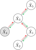
Notice that some of the (purple) message paths used to compute are the same as some of the (red) message paths used to compute —namely, any pair of red and purple paths in Fig. 5.2b that start from the same leaf. (In this example, such paths are only one edge long, but in general they could be longer). This suggests some immediate computational savings. But we can save more. We have just seen that any singleton marginal (or conditional) can be computed efficiently by treating the corresponding node in the graph as the root of a tree, and then eliminating recursively from leaves to root. Let us call this a collection for the target node. Now, if we have an arrow in both directions on every edge of the tree (Fig. 5.2c)—if we have passed a message in both directions—then we can construct collections for any node in the graph. (You should convince yourself that this is the case.)
Is it possible to compute efficiently all the messages in Fig. 5.2c, i.e. all the messages on the tree? Yes: We have already seen how to compute the red messages: a recursive collection of messages from leaves to root. The green messages, for their part, can be computed by a recursive distribution of messages from root to leaves, using the same message formula, Eq. 5.10. Note that in this case, the expression means “all neighbors of other than , to which the message is sent” (rather than “all children…”). Thus, at twice the cost of VE, belief propagation††margin: belief propagation can compute all the singleton marginals. (Pseudo-code for the entire algorithm is shown in Algorithm LABEL:alg:BP.)
For concreteness, we make this explicit for the example we have been working with. In code, we would have (picking up where we left off)
# outward pass (distribute from root, node 5)
omega53 = p_X5givenX3
assert omega53.shape == (1, 1, 2, 1, 2)
m53 = omega53.sum(axis=4, keepdims=True) # = 1
omega34 = p_X4givenX3*m53*m13
assert omega34.shape == (1, 1, 2, 2, 1)
m34 = omega34.sum(axis=2, keepdims=True) # = p(X4)
omega31 = p_X3givenX1*m43*m53
assert omega31.shape == (2, 1, 2, 1, 1)
m31 = omega31.sum(axis=2, keepdims=True) # = p(X4=1|X1)
omega12 = p_X1*p_X2givenX1*m31
assert omega12.shape == (2, 2, 1, 1, 1)
m12 = omega12.sum(axis=0, keepdims=True) # = p(X1,X4=1)
It is a simple exercise††margin: Exercise LABEL:ex: to show that Eq. 5.11 turns all these messages (including those from the inward pass) into the singleton marginals.
Finally, although we have described the message passing in belief propagation as a two-stage algorithm—collection from leaves to root, followed by distribution from root to leaves—it can be more succinctly summarized in one line:
Message-passing protocol: A node can pass a message to a neighbor once it has received messages from all its other neighbors.
To see that this is more general than the collection-distribution implementation of Algorithm LABEL:alg:BP, consider that it can also be implemented asynchronously…..
5.3.1 Belief propagation on a clique tree.
Belief propagation is elegant and efficient, but it is restricted to trees.88 8 And some “tree-like” graphs, see e.g. [35]. We would like to generalize this message-passing protocol from trees to clique trees. We attack this now.
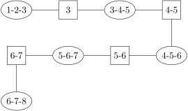
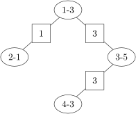
To see the connection to message passing on trees, we begin with a clique tree derived from the directed tree with which we have been working (reproduced as Fig. 5.3a). To construct this clique tree, we follow the procedure of Section 5.2, interpreting the computation of one singleton conditional in terms of variable elimination, and then linking together nodes that represent the elimination cliques. In this case, we compute in the tree in Fig. 5.2a with the elimination ordering , i.e. according to Eq. 5.9. The resulting clique graph is shown in Fig. 5.3b. We need to assign potentials to its cliques; let us make the following assignments:
Can we run BP on this tree? One way to see that we can, and how, is to interpret each node in the clique tree, Fig. 5.3b, as corresponding to a single random variable, whose support is equal to the Cartesian product of the support of the original variables that have been grouped into this node. For example, if the original random variables are each categorically distributed over categories, we can interpret clique node (2-1) as corresponding to a single, categorical random variable that takes on one of the different possible combinations of and . Similarly, we can let take on one of the different possible combinations of and ; and so on.
From this point of view, all of the clique potentials are “singleton” potentials, since each defines constraints over precisely the clique variable itself, and we could even write them as , , etc. That is,
What would the pairwise potentials be? They would be deterministic functions that enforce that neighbors match on their shared subcomponents. Let us express this very pedantically in order to derive the update equations purely mechanically:
which says that the clique variables must match on their subcomponents. For example, the nodes (2-1) and (1-3) of the clique graph in Fig. 5.3b would be governed by a “pairwise potential” of the form
With these definitions for the pairwise and singleton marginals on a clique tree in hand (Eqs. 5.13 and 5.14), we can now apply the equation for message computation, Eq. 5.10. For example, treating node (2-1) as a leaf, and therefore with no incoming messages, Eq. 5.10 tells us that the outgoing message to (1-3) is
In short, we might as well just use the original symbols, and write
Evidently, then, the generic message computation on the clique tree is
We can adjust similarly Eq. 5.11 for computing the (possibly unnormalized) marginal probabilites—now over cliques (in the present case, pairs of variables), rather than singletons:
Generalizing to other clique trees.
In sum, we have shown that a tree can be transformed into a clique tree, on which belief propagation runs with essentially no alteration to compute (clique) marginal probabilities. But it turns out that starting with a tree, although sufficient, is not necessary, so long as we end up with a clique tree with a certain locality property. There are two key insights:
- •
-
•
However, the clique tree is a tree in clique variables, , so it does not automatically come with the right guarantees about the underlying variables, . We need to ensure an additional property holds on the clique tree in order to underwrite those guarantees.
To understand this property, consider again the derivation of Eq. 5.10 in particular. To map it onto the process of variable elimination (in Eq. 5.9), we reasoned that “since the graph is a tree, the only other potentials that can reference must be its children, which by hypothesis have already been eliminated, and therefore have sent their messages .” But this does not hold for any clique tree whatsoever.
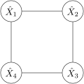
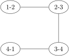
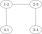
Consider, for example, the four-node, undirected cycle shown in Fig. 5.4a, and a corresponding clique tree, Fig. 5.4b. Under Eq. 5.15, a message sent from node (1-2) to (2-3) will make no reference to node (4-1). But this breaks the connection with variable elimination (the ultimate justification for our procedure), in which the summation over would not have been able to push past .
From a certain point of view, Fig. 5.4b is not a genuine clique tree, since it ignores the deterministic “potentials” defined by Eq. 5.14. It seems reasonable to require that clique nodes that are related by such a potential—i.e., that make reference to the same underlying variable —be neighbors in the graph. But this does not provide a direct solution to our problem: There is no choice of edges in Fig. 5.4b that will satisfy this demand (see e.g. Fig. 5.4c), so clearly there is more work to be done. Furthermore, it will turn out that requiring cliques that make reference to the same random variables to be neighbors is overly restrictive.
The precise form of the desired property, and constructing trees that have it, will be the subject of Section 5.4. For now we content ourselves with the conclusion that, if we can generate trees with it, then we can compute clique marginals with a lightly modified form of Eqs. 5.15 and 5.16 (modified because the cliques can have size larger than two). This is known as the Shafer-Shenoy algorithm††margin: Shafer-Shenoy algorithm [XXX], and is now thought of as one possible instantiation of the junction-tree algorithm.
In the next section (Section 5.4), we develop the “compilation phase” of the junction-tree algorithm, namely, constructing junction trees. But we will not further describe the “computation phase” in terms of the Shafer-Shenoy algorithm, since we have already discussed all of the central ingredients. Instead, we will return to the description in terms of the separator potentials we introduced in our discussion of variable elimination, Section 5.2. To set the stage for this, we consider the relationship between the messages passed on the clique tree in our example, Fig. 5.3, and the separator potentials.
5.3.2 The relationship between clique messages and sepatator potentials
The clique tree in Fig. 5.3b did not have many branches, but consider the clique-tree fragment in Fig. 5.5. Computing the message from the node (7-8) to (for example) the node (7-1) according to Eq. 5.15 means (broadcast) multiplying over all the the other messages into (7-8). But computing the message from (7-8) to (for example) the node (7-2) involves almost all of the same products! Clearly, we can save some computation if we simply precompute the product over all incoming messages, and then divide out the message from (7-) before sending one (back) out to (7-).
Under this procedure, in addition to storing the product of messages, we would have to keep around each individual one (to be able to divide it out), so there is an additional storage cost. Conceptually, let us assign the storage of the former to the node itself—in this case, (7-8), i.e.,
Notice that this is, by Eq. 5.16, precisely the (possibly unnormalized) clique marginal. Now let us furthermore assign the storage of the incoming individual messages to the separator potentials (omitted from Fig. 5.5 to save space):
Then according to Eq. 5.15, the outgoing message from (7-8) to (7-1) would be
where the last line follows from the update rule for separator potentials, Eq. 5.7. Recalling that the initial separator potentials are defined to be 1, we see that the messages passed by the Shafer-Shenoy algorithm on the clique tree are precisely the ratios of separator potentials, before and after updating.