12.3 Contrastive losses

Let us now consider a very different approach to fitting EBMs. We set aside latent variables and sampling, and only attempt to address the second of the difficulties besetting energy-based models (enumerated at the beginning of this chapter): computing the partition function. Rather than attempting to estimate the normalizer or its derivative with sample averages, we entertain a radically different approach: designing a loss function that is minimized only for an energy corresponding to a normalized distribution, i.e. for which the optimal energy satifies

∫𝒚exp⁡{−U^⁢(𝒚,𝜽)}⁢d𝒚=1.\int_{\bm{y}{}}\exp\mathopen{}\mathclose{{}\left\{-\hat{U}\mathopen{}% \mathclose{{}\left(\bm{y},\bm{\theta}}\right)}\right\}\mathop{}\!\mathrm{d}{% \bm{y}{}}=1.

We will not constrain the energy itself; that is, there exist settings of the parameters 𝜽\bm{\theta} for which this equation does not hold. However, none of these settings minimizes the loss. What objectives have this property?

12.3.1 Noise-Contrastive Estimation

The basic intuition behind noise-contrastive estimation (NCE) [19] is that one such objective is distinguishing data from noise. More precisely, we let the task be to discriminate good or “positive” samples drawn from p⁢(𝒚){p\mathopen{}\mathclose{{}\left({\color[rgb]{.75,0,.25}\definecolor[named]{% pgfstrokecolor}{rgb}{.75,0,.25}\bm{y}}}\right)} from “negative” drawn from a “noise” distribution, pn⁢(𝒚){p_{\text{n}}\mathopen{}\mathclose{{}\left({\color[rgb]{.75,0,.25}\definecolor% [named]{pgfstrokecolor}{rgb}{.75,0,.25}\bm{y}}}\right)}, by improving an unnormalized model exp⁡{−U^⁢(𝒚,𝜽)}\exp\mathopen{}\mathclose{{}\left\{-\hat{U}\mathopen{}\mathclose{{}\left({% \color[rgb]{.75,0,.25}\definecolor[named]{pgfstrokecolor}{rgb}{.75,0,.25}\bm{y% }},\bm{\theta}}\right)}\right\} for the “positive” data. The dual demands of minimizing both false alarms and misses will prevent the model from making its implicit normalizer either too big or too small (respectively). We choose the noise distribution, so we can (to some extent) control how hard this task is.

Mathematically, if X{X} is the Bernoulli random variable indicating from which of the distributions 𝒀{\bm{Y}}{} was drawn, the problem becomes that of minimizing the posterior relative entropy, DKL{p(X|𝒀)∥p^(X|𝒀;𝜽)}\operatorname*{\text{D}_{\text{KL}}}\mathopen{}\mathclose{{}\left\{{p\mathopen% {}\mathclose{{}\left({X}\middle|{\bm{Y}}}\right)}\middle\|{\hat{p}\mathopen{}% \mathclose{{}\left({X}\middle|{\bm{Y}};\bm{\theta}}\right)}}\right\}. There is no reason to make negative or positive samples more common, so we let the prior probability of X{X} be uniform. Therefore the data distribution is

equation (12.19) (12.19)
p⁢(x)\displaystyle{p\mathopen{}\mathclose{{}\left({\color[rgb]{.75,0,.25}% \definecolor[named]{pgfstrokecolor}{rgb}{.75,0,.25}x}}\right)}
. . =1/2\displaystyle{}\mathrel{\vbox{\hbox{.}\hbox{.} }}=1/2
p(𝒚|x)\displaystyle{p\mathopen{}\mathclose{{}\left({\color[rgb]{.75,0,.25}% \definecolor[named]{pgfstrokecolor}{rgb}{.75,0,.25}\bm{y}}\middle|{\color[rgb]% {.75,0,.25}\definecolor[named]{pgfstrokecolor}{rgb}{.75,0,.25}x}}\right)}
. . =p(𝒚)xpn(𝒚)1−x,\displaystyle{}\mathrel{\vbox{\hbox{.}\hbox{.} }}={p\mathopen{}\mathclose{{}\left({\color[rgb]{.75,0,.25}\definecolor[named]{% pgfstrokecolor}{rgb}{.75,0,.25}\bm{y}}}\right)}^{{\color[rgb]{.75,0,.25}% \definecolor[named]{pgfstrokecolor}{rgb}{.75,0,.25}x}}{p_{\text{n}}\mathopen{}% \mathclose{{}\left({\color[rgb]{.75,0,.25}\definecolor[named]{pgfstrokecolor}{% rgb}{.75,0,.25}\bm{y}}}\right)}^{1-{\color[rgb]{.75,0,.25}\definecolor[named]{% pgfstrokecolor}{rgb}{.75,0,.25}x}},

making the data posterior be

equation (12.20) (12.20)
p(X^=1|𝒚)=p⁢(𝒚)p⁢(𝒚)+pn⁢(𝒚).{p\mathopen{}\mathclose{{}\left({\hat{X}}=1\middle|{\color[rgb]{.75,0,.25}% \definecolor[named]{pgfstrokecolor}{rgb}{.75,0,.25}\bm{y}}}\right)}=\frac{{p% \mathopen{}\mathclose{{}\left({\color[rgb]{.75,0,.25}\definecolor[named]{% pgfstrokecolor}{rgb}{.75,0,.25}\bm{y}}}\right)}}{{p\mathopen{}\mathclose{{}% \left({\color[rgb]{.75,0,.25}\definecolor[named]{pgfstrokecolor}{rgb}{% .75,0,.25}\bm{y}}}\right)}+{p_{\text{n}}\mathopen{}\mathclose{{}\left({\color[% rgb]{.75,0,.25}\definecolor[named]{pgfstrokecolor}{rgb}{.75,0,.25}\bm{y}}}% \right)}}.

We will give our generative model the same form, except that our model for the positive data will not be normalized. For notational symmetry between the model and noise distribution, we also write the noise distribution in terms of an energy,

Un(𝒚) . . =−logpn(𝒚).U_{\text{n}}\mathopen{}\mathclose{{}\left({\color[rgb]{.75,0,.25}\definecolor[% named]{pgfstrokecolor}{rgb}{.75,0,.25}\bm{y}}}\right)\mathrel{\vbox{\hbox{.}% \hbox{.} }}=-\log{p_{\text{n}}\mathopen{}\mathclose{{}\left({\color[rgb]{.75,0,.25}% \definecolor[named]{pgfstrokecolor}{rgb}{.75,0,.25}\bm{y}}}\right)}.

Note well, however, that we define this energy to be normalized, i.e. to yield a (normalized) distribution when exponentiated. Our generative model is then

equation (12.21) (12.21)
p^⁢(x;𝜽)\displaystyle{\hat{p}\mathopen{}\mathclose{{}\left({\color[rgb]{.75,0,.25}% \definecolor[named]{pgfstrokecolor}{rgb}{.75,0,.25}x};\bm{\theta}}\right)}
. . =1/2,\displaystyle{}\mathrel{\vbox{\hbox{.}\hbox{.} }}=1/2,
q^(𝒚|x;𝜽)\displaystyle{\hat{q}\mathopen{}\mathclose{{}\left({\color[rgb]{.75,0,.25}% \definecolor[named]{pgfstrokecolor}{rgb}{.75,0,.25}\bm{y}}\middle|{\color[rgb]% {.75,0,.25}\definecolor[named]{pgfstrokecolor}{rgb}{.75,0,.25}x};\bm{\theta}}% \right)}
. . =exp{−xU^(𝒚,𝜽)−(1−x)Un(𝒚)}.\displaystyle{}\mathrel{\vbox{\hbox{.}\hbox{.} }}=\exp\mathopen{}\mathclose{{}\left\{-{\color[rgb]{.75,0,.25}\definecolor[% named]{pgfstrokecolor}{rgb}{.75,0,.25}x}\hat{U}\mathopen{}\mathclose{{}\left({% \color[rgb]{.75,0,.25}\definecolor[named]{pgfstrokecolor}{rgb}{.75,0,.25}\bm{y% }},\bm{\theta}}\right)-(1-{\color[rgb]{.75,0,.25}\definecolor[named]{% pgfstrokecolor}{rgb}{.75,0,.25}x})U_{\text{n}}\mathopen{}\mathclose{{}\left({% \color[rgb]{.75,0,.25}\definecolor[named]{pgfstrokecolor}{rgb}{.75,0,.25}\bm{y% }}}\right)}\right\}.

Now, q^(𝒚|X^=1;𝜽){\hat{q}\mathopen{}\mathclose{{}\left({\color[rgb]{.75,0,.25}\definecolor[% named]{pgfstrokecolor}{rgb}{.75,0,.25}\bm{y}}\middle|{\hat{X}}=1;\bm{\theta}}% \right)} is not normalized: at the beginning of training, at least, it will not integrate to 1. Nevertheless, if we ignore this and compute the posterior in the usual way with Bayes’ rule, we get a perfectly legitimate probability distribution. In particular, the posterior probability of an example being positive is

equation (12.22) (12.22)
p^(X^=1|𝒚;𝜽)=exp⁡{−U^⁢(𝒚,𝜽)}exp⁡{−U^⁢(𝒚,𝜽)}+exp⁡{−Un⁢(𝒚)}=σ{Un(𝒚)−U^(𝒚,𝜽)}=σ{h(𝒚,𝜽)},{\hat{p}\mathopen{}\mathclose{{}\left({\hat{X}}=1\middle|{\color[rgb]{% .75,0,.25}\definecolor[named]{pgfstrokecolor}{rgb}{.75,0,.25}\bm{y}};\bm{% \theta}}\right)}=\frac{\exp\mathopen{}\mathclose{{}\left\{-\hat{U}\mathopen{}% \mathclose{{}\left({\color[rgb]{.75,0,.25}\definecolor[named]{pgfstrokecolor}{% rgb}{.75,0,.25}\bm{y}},\bm{\theta}}\right)}\right\}}{\exp\mathopen{}\mathclose% {{}\left\{-\hat{U}\mathopen{}\mathclose{{}\left({\color[rgb]{.75,0,.25}% \definecolor[named]{pgfstrokecolor}{rgb}{.75,0,.25}\bm{y}},\bm{\theta}}\right)% }\right\}+\exp\mathopen{}\mathclose{{}\left\{-U_{\text{n}}\mathopen{}% \mathclose{{}\left({\color[rgb]{.75,0,.25}\definecolor[named]{pgfstrokecolor}{% rgb}{.75,0,.25}\bm{y}}}\right)}\right\}}=\sigma\mathopen{}\mathclose{{}\left\{% U_{\text{n}}\mathopen{}\mathclose{{}\left({\color[rgb]{.75,0,.25}\definecolor[% named]{pgfstrokecolor}{rgb}{.75,0,.25}\bm{y}}}\right)-\hat{U}\mathopen{}% \mathclose{{}\left({\color[rgb]{.75,0,.25}\definecolor[named]{pgfstrokecolor}{% rgb}{.75,0,.25}\bm{y}},\bm{\theta}}\right)}\right\}=\sigma\mathopen{}% \mathclose{{}\left\{h\mathopen{}\mathclose{{}\left({\color[rgb]{.75,0,.25}% \definecolor[named]{pgfstrokecolor}{rgb}{.75,0,.25}\bm{y}},\bm{\theta}}\right)% }\right\},

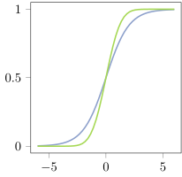
with σ\sigma the logistic function and h⁢(𝒚,𝜽)h\mathopen{}\mathclose{{}\left({\color[rgb]{.75,0,.25}\definecolor[named]{% pgfstrokecolor}{rgb}{.75,0,.25}\bm{y}},\bm{\theta}}\right) the difference in energies:

equation (12.23) (12.23)
h(𝒚,𝜽) . . =Un(𝒚)−U^(𝒚,𝜽).h\mathopen{}\mathclose{{}\left({\color[rgb]{.75,0,.25}\definecolor[named]{% pgfstrokecolor}{rgb}{.75,0,.25}\bm{y}},\bm{\theta}}\right)\mathrel{\vbox{\hbox% {.}\hbox{.} }}=U_{\text{n}}\mathopen{}\mathclose{{}\left({\color[rgb]{.75,0,.25}% \definecolor[named]{pgfstrokecolor}{rgb}{.75,0,.25}\bm{y}}}\right)-\hat{U}% \mathopen{}\mathclose{{}\left({\color[rgb]{.75,0,.25}\definecolor[named]{% pgfstrokecolor}{rgb}{.75,0,.25}\bm{y}},\bm{\theta}}\right).

The key result that makes NCE work is that the relative entropy of this posterior is minimized only when U^⁢(𝒚,𝜽)=−log⁡p⁢(𝒚)\hat{U}\mathopen{}\mathclose{{}\left({\color[rgb]{.75,0,.25}\definecolor[named% ]{pgfstrokecolor}{rgb}{.75,0,.25}\bm{y}},\bm{\theta}}\right)=-\log{p\mathopen{% }\mathclose{{}\left({\color[rgb]{.75,0,.25}\definecolor[named]{pgfstrokecolor}% {rgb}{.75,0,.25}\bm{y}}}\right)}, as opposed to U^⁢(𝒚,𝜽)=−log⁡p⁢(𝒚)+C\hat{U}\mathopen{}\mathclose{{}\left({\color[rgb]{.75,0,.25}\definecolor[named% ]{pgfstrokecolor}{rgb}{.75,0,.25}\bm{y}},\bm{\theta}}\right)=-\log{p\mathopen{% }\mathclose{{}\left({\color[rgb]{.75,0,.25}\definecolor[named]{pgfstrokecolor}% {rgb}{.75,0,.25}\bm{y}}}\right)}+C for some constant CC. To see this, note that relative entropy is minimized when the data and model posteriors are equal; or, from Eqs. 12.20 and 12.22, when

σ⁢{Un⁢(𝒚)−U^⁢(𝒚,𝜽)}=setp⁢(𝒚)p⁢(𝒚)+pn⁢(𝒚)=σ⁢{log⁡(p⁢(𝒚)pn⁢(𝒚))}.\begin{split}\sigma\mathopen{}\mathclose{{}\left\{U_{\text{n}}\mathopen{}% \mathclose{{}\left({\color[rgb]{.75,0,.25}\definecolor[named]{pgfstrokecolor}{% rgb}{.75,0,.25}\bm{y}}}\right)-\hat{U}\mathopen{}\mathclose{{}\left({\color[% rgb]{.75,0,.25}\definecolor[named]{pgfstrokecolor}{rgb}{.75,0,.25}\bm{y}},\bm{% \theta}}\right)}\right\}\stackrel{{\scriptstyle\text{set}}}{{=}}\frac{{p% \mathopen{}\mathclose{{}\left({\color[rgb]{.75,0,.25}\definecolor[named]{% pgfstrokecolor}{rgb}{.75,0,.25}\bm{y}}}\right)}}{{p\mathopen{}\mathclose{{}% \left({\color[rgb]{.75,0,.25}\definecolor[named]{pgfstrokecolor}{rgb}{% .75,0,.25}\bm{y}}}\right)}+{p_{\text{n}}\mathopen{}\mathclose{{}\left({\color[% rgb]{.75,0,.25}\definecolor[named]{pgfstrokecolor}{rgb}{.75,0,.25}\bm{y}}}% \right)}}=\sigma\mathopen{}\mathclose{{}\left\{\log\mathopen{}\mathclose{{}% \left(\frac{{p\mathopen{}\mathclose{{}\left({\color[rgb]{.75,0,.25}% \definecolor[named]{pgfstrokecolor}{rgb}{.75,0,.25}\bm{y}}}\right)}}{{p_{\text% {n}}\mathopen{}\mathclose{{}\left({\color[rgb]{.75,0,.25}\definecolor[named]{% pgfstrokecolor}{rgb}{.75,0,.25}\bm{y}}}\right)}}}\right)}\right\}.\end{split}

Clearly this requires U^⁢(𝒚,𝜽)=−log⁡p⁢(𝒚)\hat{U}\mathopen{}\mathclose{{}\left({\color[rgb]{.75,0,.25}\definecolor[named% ]{pgfstrokecolor}{rgb}{.75,0,.25}\bm{y}},\bm{\theta}}\right)=-\log{p\mathopen{% }\mathclose{{}\left({\color[rgb]{.75,0,.25}\definecolor[named]{pgfstrokecolor}% {rgb}{.75,0,.25}\bm{y}}}\right)}.99 9 Technically, the proof requires the noise distribution to be supported wherever the data distribution is [19]. So we will not need to compute the normalizer, i.e. to integrate U^⁢(𝒚,𝜽)\hat{U}\mathopen{}\mathclose{{}\left({\color[rgb]{.75,0,.25}\definecolor[named% ]{pgfstrokecolor}{rgb}{.75,0,.25}\bm{y}},\bm{\theta}}\right). Intuitively, this happens because the model and noise energies always show up together and must balance. If the learned (implicit) normalizer is too small, for example if the model energy U^⁢(𝒚,𝜽)\hat{U}\mathopen{}\mathclose{{}\left({\color[rgb]{.75,0,.25}\definecolor[named% ]{pgfstrokecolor}{rgb}{.75,0,.25}\bm{y}},\bm{\theta}}\right) is smaller than the noise energy for most values of 𝒚{\color[rgb]{.75,0,.25}\definecolor[named]{pgfstrokecolor}{rgb}{.75,0,.25}\bm{% y}}, then most negative samples will be assigned to the positive distribution. The reverse, also undesirable, holds when the implicit normalizer is too large. Both kinds of mistakes will increase the relative entropy.

Notice, however, that these mistakes will be less noticeable if the data and noise distributions are very different from each other—e.g., if the bulks of the probability masses of the distributions are very far from each other. In this case, the model could assign (e.g.) overly high probability to the data (by making the normalizer too small) without making the noise samples particularly probable under the model. Technically, the normalized energy of the data distribution is guaranteed to be the unique solution to the loss based on the posterior in Eq. 12.22 (see below) as long as the noise distribution is supported wherever the data distribution is. But for finite training samples (the situation in which we usually find ourselves), the guarantee is voided. The problem would appear to be more acute for more expressive model distributions.

Quasi-generative learning.

The relative entropy of the posterior distributions of the data and model—Eqs. 12.20 and 12.22, respectively—is

equation (12.24) (12.24)
ℒ︀=DKL{p(X|𝒀)∥p^(X|𝒀;𝜽)}≈+⟨−log(p^(X^=1|𝒀;𝜽)Xp^(X^=0|𝒀;𝜽)1−X)⟩X,𝒀=12⟨−logp^(X^=1|𝒀+;𝜽)⟩𝒀++12⟨−log(1−p^(X^=1|𝒀−;𝜽))⟩𝒀−=12⁢⟨−log⁡σ⁢{h⁢(𝒀+,𝜽)}⟩𝒀++12⁢⟨−log⁡σ⁢{−h⁢(𝒀−,𝜽)}⟩𝒀−.\begin{split}\mathcal{L}&{}=\operatorname*{\text{D}_{\text{KL}}}\mathopen{}% \mathclose{{}\left\{{p\mathopen{}\mathclose{{}\left({X}\middle|{\bm{Y}}}\right% )}\middle\|{\hat{p}\mathopen{}\mathclose{{}\left({X}\middle|{\bm{Y}};\bm{% \theta}}\right)}}\right\}\\ &{}\stackrel{{\scriptstyle\text{+}}}{{\approx}}{\mathopen{}\mathclose{{}\left% \langle{-\log\mathopen{}\mathclose{{}\left({\hat{p}\mathopen{}\mathclose{{}% \left({\hat{X}}=1\middle|{\bm{Y}};\bm{\theta}}\right)}^{{X}}{\hat{p}\mathopen{% }\mathclose{{}\left({\hat{X}}=0\middle|{\bm{Y}};\bm{\theta}}\right)}^{1-{X}}}% \right)}}\right\rangle_{{X}{},{\bm{Y}}{}}}\\ &{}=\frac{1}{2}{\mathopen{}\mathclose{{}\left\langle{-\log{\hat{p}\mathopen{}% \mathclose{{}\left({\hat{X}}=1\middle|{\bm{Y}}_{+};\bm{\theta}}\right)}}}% \right\rangle_{{\bm{Y}}_{+}{}}}+\frac{1}{2}{\mathopen{}\mathclose{{}\left% \langle{-\log\mathopen{}\mathclose{{}\left(1-{\hat{p}\mathopen{}\mathclose{{}% \left({\hat{X}}=1\middle|{\bm{Y}}_{-};\bm{\theta}}\right)}}\right)}}\right% \rangle_{{\bm{Y}}_{-}{}}}\\ &{}=\frac{1}{2}{\mathopen{}\mathclose{{}\left\langle{-\log\sigma\mathopen{}% \mathclose{{}\left\{h\mathopen{}\mathclose{{}\left({\bm{Y}}_{+},\bm{\theta}}% \right)}\right\}}}\right\rangle_{{\bm{Y}}_{+}{}}}+\frac{1}{2}{\mathopen{}% \mathclose{{}\left\langle{-\log\sigma\mathopen{}\mathclose{{}\left\{-h% \mathopen{}\mathclose{{}\left({\bm{Y}}_{-},\bm{\theta}}\right)}\right\}}}% \right\rangle_{{\bm{Y}}_{-}{}}}.\end{split}

This is evidently a discriminative problem, but with a twist. The canonical generative approach to binary classification is to model the generative distribution p^(x;𝜽)p^(𝒚|x;𝜽){\hat{p}\mathopen{}\mathclose{{}\left({\color[rgb]{.75,0,.25}\definecolor[% named]{pgfstrokecolor}{rgb}{.75,0,.25}x};\bm{\theta}}\right)}{\hat{p}\mathopen% {}\mathclose{{}\left({\color[rgb]{.75,0,.25}\definecolor[named]{pgfstrokecolor% }{rgb}{.75,0,.25}\bm{y}}\middle|{\color[rgb]{.75,0,.25}\definecolor[named]{% pgfstrokecolor}{rgb}{.75,0,.25}x};\bm{\theta}}\right)} (like NCE); acquire the parameters by minimizing the joint relative entropy DKL⁡{p⁢(X,𝒀)∥p^⁢(X,𝒀;𝜽)}\operatorname*{\text{D}_{\text{KL}}}\mathopen{}\mathclose{{}\left\{{p\mathopen% {}\mathclose{{}\left({X},{\bm{Y}}}\right)}\middle\|{\hat{p}\mathopen{}% \mathclose{{}\left({X},{\bm{Y}};\bm{\theta}}\right)}}\right\} (unlike NCE); and then invert to p^(x|𝒚;𝜽){\hat{p}\mathopen{}\mathclose{{}\left({\color[rgb]{.75,0,.25}\definecolor[% named]{pgfstrokecolor}{rgb}{.75,0,.25}x}\middle|{\color[rgb]{.75,0,.25}% \definecolor[named]{pgfstrokecolor}{rgb}{.75,0,.25}\bm{y}};\bm{\theta}}\right)} with Bayes’ rule. For example, for Gaussian mixtures, this is known as linear/quadratic discriminant analysis (depending on whether the covariance is the same/different across classes). The canonical discriminative approach to binary classification is to model p^(x|𝒚;𝜽){\hat{p}\mathopen{}\mathclose{{}\left({\color[rgb]{.75,0,.25}\definecolor[% named]{pgfstrokecolor}{rgb}{.75,0,.25}x}\middle|{\color[rgb]{.75,0,.25}% \definecolor[named]{pgfstrokecolor}{rgb}{.75,0,.25}\bm{y}};\bm{\theta}}\right)} directly (unlike NCE); and then minimize the posterior relative entropy DKL{p(X|𝒀)∥p^(X|𝒀;𝜽)}\operatorname*{\text{D}_{\text{KL}}}\mathopen{}\mathclose{{}\left\{{p\mathopen% {}\mathclose{{}\left({X}\middle|{\bm{Y}}}\right)}\middle\|{\hat{p}\mathopen{}% \mathclose{{}\left({X}\middle|{\bm{Y}};\bm{\theta}}\right)}}\right\} (like NCE). This is logistic regression. NCE mixes both methods: it models the generative distribution p^(x;𝜽)p^(𝒚|x;𝜽){\hat{p}\mathopen{}\mathclose{{}\left({\color[rgb]{.75,0,.25}\definecolor[% named]{pgfstrokecolor}{rgb}{.75,0,.25}x};\bm{\theta}}\right)}{\hat{p}\mathopen% {}\mathclose{{}\left({\color[rgb]{.75,0,.25}\definecolor[named]{pgfstrokecolor% }{rgb}{.75,0,.25}\bm{y}}\middle|{\color[rgb]{.75,0,.25}\definecolor[named]{% pgfstrokecolor}{rgb}{.75,0,.25}x};\bm{\theta}}\right)}, but first inverts with Bayes rule, and finally minimizes the posterior relative entropy DKL{p(X|𝒀)∥p^(X|𝒀;𝜽)}\operatorname*{\text{D}_{\text{KL}}}\mathopen{}\mathclose{{}\left\{{p\mathopen% {}\mathclose{{}\left({X}\middle|{\bm{Y}}}\right)}\middle\|{\hat{p}\mathopen{}% \mathclose{{}\left({X}\middle|{\bm{Y}};\bm{\theta}}\right)}}\right\}. In the classic case of the mixture of two Gaussians/binary classification, this would amount to learning the two (mean, covariance) pairs by minimizing the posterior relative entropy—as opposed to learning these parameters by minimizing the joint relative entropy (generative), or learning a separating hyperplane by minimizing the posterior relative entropy (discriminative). These contrasts are summarized in Table 12.1.††margin: Nice properties of the estimator….

generative classifier discriminative classifier NCE
loss DKL⁡{p⁢(X,𝒀)∥p^⁢(X,𝒀;𝜽)}\operatorname*{\text{D}_{\text{KL}}}\mathopen{}\mathclose{{}\left\{{p\mathopen% {}\mathclose{{}\left({X},{\bm{Y}}}\right)}\middle\|{\hat{p}\mathopen{}% \mathclose{{}\left({X},{\bm{Y}};\bm{\theta}}\right)}}\right\} DKL{p(X|𝒀)∥p^(X|𝒀;𝜽)}\operatorname*{\text{D}_{\text{KL}}}\mathopen{}\mathclose{{}\left\{{p\mathopen% {}\mathclose{{}\left({X}\middle|{\bm{Y}}}\right)}\middle\|{\hat{p}\mathopen{}% \mathclose{{}\left({X}\middle|{\bm{Y}};\bm{\theta}}\right)}}\right\} DKL{p(X|𝒀)∥p^(X|𝒀;𝜽)}\operatorname*{\text{D}_{\text{KL}}}\mathopen{}\mathclose{{}\left\{{p\mathopen% {}\mathclose{{}\left({X}\middle|{\bm{Y}}}\right)}\middle\|{\hat{p}\mathopen{}% \mathclose{{}\left({X}\middle|{\bm{Y}};\bm{\theta}}\right)}}\right\}
model p^(𝒙;𝜽)p^(𝒚|𝒙;𝜽){\hat{p}\mathopen{}\mathclose{{}\left({\color[rgb]{.75,0,.25}\definecolor[% named]{pgfstrokecolor}{rgb}{.75,0,.25}\bm{x}}{};\bm{\theta}}\right)}{\hat{p}% \mathopen{}\mathclose{{}\left({\color[rgb]{.75,0,.25}\definecolor[named]{% pgfstrokecolor}{rgb}{.75,0,.25}\bm{y}}\middle|{\color[rgb]{.75,0,.25}% \definecolor[named]{pgfstrokecolor}{rgb}{.75,0,.25}\bm{x}}{};\bm{\theta}}% \right)} p^(𝒙|𝒚;𝜽){\hat{p}\mathopen{}\mathclose{{}\left({\color[rgb]{.75,0,.25}\definecolor[% named]{pgfstrokecolor}{rgb}{.75,0,.25}\bm{x}}{}\middle|{\color[rgb]{.75,0,.25}% \definecolor[named]{pgfstrokecolor}{rgb}{.75,0,.25}\bm{y}};\bm{\theta}}\right)} p^(𝒙;𝜽)p^(𝒚|𝒙;𝜽){\hat{p}\mathopen{}\mathclose{{}\left({\color[rgb]{.75,0,.25}\definecolor[% named]{pgfstrokecolor}{rgb}{.75,0,.25}\bm{x}}{};\bm{\theta}}\right)}{\hat{p}% \mathopen{}\mathclose{{}\left({\color[rgb]{.75,0,.25}\definecolor[named]{% pgfstrokecolor}{rgb}{.75,0,.25}\bm{y}}\middle|{\color[rgb]{.75,0,.25}% \definecolor[named]{pgfstrokecolor}{rgb}{.75,0,.25}\bm{x}}{};\bm{\theta}}% \right)}
Bayes’ rule? during inference never during training
use discrimination discrimination density estimation
Table 12.1: Comparison of learning algorithms for mixture models

12.3.2 InfoNCE

Van den Oord and colleagues propose to put NCE to a very different purpose [75]. Rather than attempting to learn a parametric form for the probability of observed samples, they aim to extract useful features from data. In order to do so, they introduce what amounts to four novel variations on NCE, which we discuss one at a time below.

At an abstract level, the approach can be described as follows. Our goal is to make the relationship between two variables more perspicuous—or, more technically, more accessible to a linear function. The variables might be, for example, two views of the same object. Rather than learn to discriminate data samples from noise samples, as in NCE, we will learn to discriminate pairs of samples that are related to each other from pairs of samples that are not. The procedure is the same: we draw samples either from a joint distribution over dependent variables, or from a pair of marginal distributions over independent variables—labeled as such—and minimize the posterior relative entropy. In our example, we draw either two views of the same object or two views of two different objects.

Since our goal is not to assign energies to samples (or to generate them), we do not model the energy of the joint distribution (or of the product of marginals). Instead, our goal is to learn a feature space in which the relationship between the varaibles is simple. Accordingly, we model the difference of energies as (prototypically) an inner product of the features of the two samples. In learning to discriminate on the basis of this difference in energies, the model learns to make two views of the same object have a large inner product, and two views of different objects have a small inner product.

Why use an inner product? If training is successful, what is common between two views of the same object will be contained only this inner product. This feature of the data can therefore be read out with a linear operation—that is, the sufficient statistic is linear.

(1) Generalizing to multiple “examples.”

Suppose that the observation 𝒚\bm{y} is not a single sample but a collection of K{K} “examples,” (𝒚1,…,𝒚K(\bm{y}_{1},\ldots,\bm{y}_{{K}}), precisely one of which is not noise. Then the goal is not to determine whether or not the sample is noise, but rather to determine which of the examples is noise. This means that rather than use the model-noise energy difference (Eq. 12.23) directly to assign the example to the positive or negative class, as in NCE, we will compare K{K} energy differences to each other (with the softmax function).
a
b
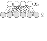
Figure 12.2: Generalizations of NCE for representation learning. (12.2a) InfoNCE. For each toss of a K{K}-sided die, 𝑿^{\bm{\hat{X}}}{}, one sample (corresponding to the face of the die that came up) is drawn from the model distribution, and K−1{K}-1 samples are drawn from a noise distribution. (12.2b) “Local NCE” (as in wav2vec). For each of N{N} trials, a coin is flipped K{K} times to determine whether to draw data from the model distribution or a noise distribution. Note that the data distribution is the same for both models, and corresponds to (12.2a), with q^⁢(𝒚;𝜽){\hat{q}\mathopen{}\mathclose{{}\left({\color[rgb]{.75,0,.25}\definecolor[% named]{pgfstrokecolor}{rgb}{.75,0,.25}\bm{y}};\bm{\theta}}\right)} replaced by the data (Eq. 12.25).

In this setup, the latent variable is categorical (conceived as a one-hot vector 𝑿^{\bm{\hat{X}}}) rather than Bernoulli, and the data distribution is:

equation (12.25) (12.25)
p⁢(𝒙)\displaystyle{p\mathopen{}\mathclose{{}\left({\color[rgb]{.75,0,.25}% \definecolor[named]{pgfstrokecolor}{rgb}{.75,0,.25}\bm{x}}{}}\right)}
=1K,\displaystyle{}=\frac{1}{{K}},
p(𝒚1,…,𝒚K|𝒙)\displaystyle{p\mathopen{}\mathclose{{}\left({\color[rgb]{.75,0,.25}% \definecolor[named]{pgfstrokecolor}{rgb}{.75,0,.25}\bm{y}_{1}},\ldots,{\color[% rgb]{.75,0,.25}\definecolor[named]{pgfstrokecolor}{rgb}{.75,0,.25}\bm{y}_{{K}}% }\middle|{\color[rgb]{.75,0,.25}\definecolor[named]{pgfstrokecolor}{rgb}{% .75,0,.25}\bm{x}}{}}\right)}
=∏k=1Kp⁢(𝒚k)xk⁢pn⁢(𝒚k)1−xk.\displaystyle{}=\prod_{k=1}^{{K}}{p\mathopen{}\mathclose{{}\left({\color[rgb]{% .75,0,.25}\definecolor[named]{pgfstrokecolor}{rgb}{.75,0,.25}\bm{y}_{k}}}% \right)}^{{\color[rgb]{.75,0,.25}\definecolor[named]{pgfstrokecolor}{rgb}{% .75,0,.25}x_{k}}}{p_{\text{n}}\mathopen{}\mathclose{{}\left({\color[rgb]{% .75,0,.25}\definecolor[named]{pgfstrokecolor}{rgb}{.75,0,.25}\bm{y}_{k}}}% \right)}^{1-{\color[rgb]{.75,0,.25}\definecolor[named]{pgfstrokecolor}{rgb}{% .75,0,.25}x_{k}}}.

Again we have set the prior uniform, since we have no reason to make any one of the elements more or less likely to be noise than any other. We emphasize that this is not a mixture model: a single sample contains K{K} “examples”: one positive, and K−1{K}-1 negative.

The generative model takes the same form, with the model distribution taking the place of the data marginal. Writing it in terms of energies, we obtain

p^⁢(𝒙;𝜽)\displaystyle{\hat{p}\mathopen{}\mathclose{{}\left({\color[rgb]{.75,0,.25}% \definecolor[named]{pgfstrokecolor}{rgb}{.75,0,.25}\bm{x}}{};\bm{\theta}}% \right)}
=1K,\displaystyle{}=\frac{1}{{K}},
q^(𝒚1,…,𝒚K|𝒙;𝜽)\displaystyle{\hat{q}\mathopen{}\mathclose{{}\left({\color[rgb]{.75,0,.25}% \definecolor[named]{pgfstrokecolor}{rgb}{.75,0,.25}\bm{y}_{1}},\ldots,{\color[% rgb]{.75,0,.25}\definecolor[named]{pgfstrokecolor}{rgb}{.75,0,.25}\bm{y}_{{K}}% }\middle|{\color[rgb]{.75,0,.25}\definecolor[named]{pgfstrokecolor}{rgb}{% .75,0,.25}\bm{x}}{};\bm{\theta}}\right)}
=exp⁡{∑kK(−xk⁢U^⁢(𝒚k,𝜽)−(1−xk)⁢Un⁢(𝒚k))}.\displaystyle{}=\exp\mathopen{}\mathclose{{}\left\{\sum_{k}^{{K}}\mathopen{}% \mathclose{{}\left(-{\color[rgb]{.75,0,.25}\definecolor[named]{pgfstrokecolor}% {rgb}{.75,0,.25}x_{k}}\hat{U}\mathopen{}\mathclose{{}\left({\color[rgb]{% .75,0,.25}\definecolor[named]{pgfstrokecolor}{rgb}{.75,0,.25}\bm{y}_{k}},\bm{% \theta}}\right)-(1-{\color[rgb]{.75,0,.25}\definecolor[named]{pgfstrokecolor}{% rgb}{.75,0,.25}x_{k}})U_{\text{n}}\mathopen{}\mathclose{{}\left({\color[rgb]{% .75,0,.25}\definecolor[named]{pgfstrokecolor}{rgb}{.75,0,.25}\bm{y}_{k}}}% \right)}\right)}\right\}.

Again we ignore the fact that the emission is unnormalized and simply compute a (normalized) posterior distribution with Bayes’ rule

equation (12.26) (12.26)
p^(X^i=1|𝒚1,…,𝒚K;𝜽)=1K⁢exp⁡{−U^⁢(𝒚i,𝜽)−∑k≠iKUn⁢(𝒚k)}∑j=1K1K⁢exp⁡{−U^⁢(𝒚j,𝜽)−∑k≠jKUn⁢(𝒚k)}=1K⁢exp⁡{h⁢(𝒚i,𝜽)−∑k=1KUn⁢(𝒚k)}∑j=1K1K⁢exp⁡{h⁢(𝒚j,𝜽)−∑k=1KUn⁢(𝒚k)}=exp⁡{h⁢(𝒚i,𝜽)}∑j=1Kexp⁡{h⁢(𝒚j,𝜽)}=softmax{h(𝒚1,𝜽)…,h(𝒚K,𝜽)}i;\begin{split}{\hat{p}\mathopen{}\mathclose{{}\left({\hat{X}}_{i}=1\middle|{% \color[rgb]{.75,0,.25}\definecolor[named]{pgfstrokecolor}{rgb}{.75,0,.25}\bm{y% }_{1}},\ldots,{\color[rgb]{.75,0,.25}\definecolor[named]{pgfstrokecolor}{rgb}{% .75,0,.25}\bm{y}_{{K}}};\bm{\theta}}\right)}&{}=\frac{\frac{1}{{K}}\exp% \mathopen{}\mathclose{{}\left\{-\hat{U}\mathopen{}\mathclose{{}\left({\color[% rgb]{.75,0,.25}\definecolor[named]{pgfstrokecolor}{rgb}{.75,0,.25}\bm{y}_{i}},% \bm{\theta}}\right)-\sum_{k\neq i}^{{K}}U_{\text{n}}\mathopen{}\mathclose{{}% \left({\color[rgb]{.75,0,.25}\definecolor[named]{pgfstrokecolor}{rgb}{% .75,0,.25}\bm{y}_{k}}}\right)}\right\}}{\sum_{j=1}^{{K}}\frac{1}{{K}}\exp% \mathopen{}\mathclose{{}\left\{-\hat{U}\mathopen{}\mathclose{{}\left({\color[% rgb]{.75,0,.25}\definecolor[named]{pgfstrokecolor}{rgb}{.75,0,.25}\bm{y}_{j}},% \bm{\theta}}\right)-\sum_{k\neq j}^{{K}}U_{\text{n}}\mathopen{}\mathclose{{}% \left({\color[rgb]{.75,0,.25}\definecolor[named]{pgfstrokecolor}{rgb}{% .75,0,.25}\bm{y}_{k}}}\right)}\right\}}\\ &{}=\frac{\frac{1}{{K}}\exp\mathopen{}\mathclose{{}\left\{h\mathopen{}% \mathclose{{}\left({\color[rgb]{.75,0,.25}\definecolor[named]{pgfstrokecolor}{% rgb}{.75,0,.25}\bm{y}_{i}},\bm{\theta}}\right)-\sum_{k=1}^{{K}}U_{\text{n}}% \mathopen{}\mathclose{{}\left({\color[rgb]{.75,0,.25}\definecolor[named]{% pgfstrokecolor}{rgb}{.75,0,.25}\bm{y}_{k}}}\right)}\right\}}{\sum_{j=1}^{{K}}% \frac{1}{{K}}\exp\mathopen{}\mathclose{{}\left\{h\mathopen{}\mathclose{{}\left% ({\color[rgb]{.75,0,.25}\definecolor[named]{pgfstrokecolor}{rgb}{.75,0,.25}\bm% {y}_{j}},\bm{\theta}}\right)-\sum_{k=1}^{{K}}U_{\text{n}}\mathopen{}\mathclose% {{}\left({\color[rgb]{.75,0,.25}\definecolor[named]{pgfstrokecolor}{rgb}{% .75,0,.25}\bm{y}_{k}}}\right)}\right\}}\\ &{}=\frac{\exp\mathopen{}\mathclose{{}\left\{h\mathopen{}\mathclose{{}\left({% \color[rgb]{.75,0,.25}\definecolor[named]{pgfstrokecolor}{rgb}{.75,0,.25}\bm{y% }_{i}},\bm{\theta}}\right)}\right\}}{\sum_{j=1}^{{K}}\exp\mathopen{}\mathclose% {{}\left\{h\mathopen{}\mathclose{{}\left({\color[rgb]{.75,0,.25}\definecolor[% named]{pgfstrokecolor}{rgb}{.75,0,.25}\bm{y}_{j}},\bm{\theta}}\right)}\right\}% }\\ &{}=\operatorname*{softmax}\mathopen{}\mathclose{{}\left\{h\mathopen{}% \mathclose{{}\left({\color[rgb]{.75,0,.25}\definecolor[named]{pgfstrokecolor}{% rgb}{.75,0,.25}\bm{y}_{1}},\bm{\theta}}\right)\ldots,h\mathopen{}\mathclose{{}% \left({\color[rgb]{.75,0,.25}\definecolor[named]{pgfstrokecolor}{rgb}{% .75,0,.25}\bm{y}_{{K}}},\bm{\theta}}\right)}\right\}_{i};\end{split}

that is, the ithi^{\text{th}} output of the softmax function. Eq. 12.26 is evidently a kind of generalization of Eq. 12.22.1010 10 However, note that the multi-example version of NCE does not quite reduce to the single-example case even when K=2{K}=2. Eq. 12.22 can indeed be re-written with a softmax as in Eq. 12.26, with the first argument equal to h⁢(𝒚i,𝜽)h\mathopen{}\mathclose{{}\left({\color[rgb]{.75,0,.25}\definecolor[named]{% pgfstrokecolor}{rgb}{.75,0,.25}\bm{y}_{i}},\bm{\theta}}\right) and the second equal to 0. The latter reflects our indifferent prior, which provides no additional information. In the two-example version of the generalization under discussion, on the other hand, the second argument encodes the relative probability of the second example being data or noise. In short, deciding which of two samples is “real” is easier than deciding whether or not a single sample is. Putting this together with the data distribution, we can write the posterior relative entropy as

equation (12.27) (12.27)
ℒ︀=DKL{p(𝑿|𝒀1,…,𝒀K)∥p^(𝑿|𝒀1,…,𝒀K;𝜽)}≈+⟨−log(∏k=1Kp^(Xk=1|𝒀1,…,𝒀K;𝜽)Xk)⟩𝑿,𝒀1,…,𝒀K=⟨−∑k=1KXklogp^(Xk=1|𝒀1,…,𝒀K;𝜽)⟩𝑿,𝒀1,…,𝒀K=⟨−logp^(X+=1|𝒀1,…,𝒀K;𝜽)⟩𝒀1,…,𝒀K=⟨−log(softmax{h(𝒀1,𝜽),…,h(𝒀K,𝜽)}+)⟩𝒀1,…,𝒀K.\begin{split}\mathcal{L}&{}=\operatorname*{\text{D}_{\text{KL}}}\mathopen{}% \mathclose{{}\left\{{p\mathopen{}\mathclose{{}\left({\bm{X}}\middle|{\bm{Y}}_{% 1},\ldots,{\bm{Y}}_{{K}}}\right)}\middle\|{\hat{p}\mathopen{}\mathclose{{}% \left({\bm{X}}\middle|{\bm{Y}}_{1},\ldots,{\bm{Y}}_{{K}};\bm{\theta}}\right)}}% \right\}\\ &{}\stackrel{{\scriptstyle\text{+}}}{{\approx}}{\mathopen{}\mathclose{{}\left% \langle{-\log\mathopen{}\mathclose{{}\left(\prod_{k=1}^{{K}}{\hat{p}\mathopen{% }\mathclose{{}\left({X}_{k}=1\middle|{\bm{Y}}_{1},\ldots,{\bm{Y}}_{{K}};\bm{% \theta}}\right)}^{{X}_{k}}}\right)}}\right\rangle_{{\bm{X}}{}{},{\bm{Y}}_{1},% \ldots,{\bm{Y}}_{{K}}{}}}\\ &{}={\mathopen{}\mathclose{{}\left\langle{-\sum_{k=1}^{{K}}{X}_{k}\log{\hat{p}% \mathopen{}\mathclose{{}\left({X}_{k}=1\middle|{\bm{Y}}_{1},\ldots,{\bm{Y}}_{{% K}};\bm{\theta}}\right)}}}\right\rangle_{{\bm{X}}{}{},{\bm{Y}}_{1},\ldots,{\bm% {Y}}_{{K}}{}}}\\ &{}={\mathopen{}\mathclose{{}\left\langle{-\log{\hat{p}\mathopen{}\mathclose{{% }\left({X}_{+}=1\middle|{\bm{Y}}_{1},\ldots,{\bm{Y}}_{{K}};\bm{\theta}}\right)% }}}\right\rangle_{{\bm{Y}}_{1},\ldots,{\bm{Y}}_{{K}}{}}}\\ &{}={\mathopen{}\mathclose{{}\left\langle{-\log\mathopen{}\mathclose{{}\left(% \operatorname*{softmax}\mathopen{}\mathclose{{}\left\{h\mathopen{}\mathclose{{% }\left({\bm{Y}}_{1},\bm{\theta}}\right),\ldots,h\mathopen{}\mathclose{{}\left(% {\bm{Y}}_{{K}},\bm{\theta}}\right)}\right\}_{+}}\right)}}\right\rangle_{{\bm{Y% }}_{1},\ldots,{\bm{Y}}_{{K}}{}}}.\end{split}

In the final line, we are selecting only that output of the softmax function that corresponds to the actual positive sample (whose index will of course differ from trial to trial).

Negative samples enforce normalization.

We can shed light on the role played by the negative examples by considering them separately from the positive example in the posterior probability of a positive example:

p^(X^+=1|𝒚1,…,𝒚K;𝜽)=exp⁡{h⁢(𝒚+,𝜽)}exp⁡{h⁢(𝒚+,𝜽)}+∑j≠+Kexp⁡{h⁢(𝒚j,𝜽)}.{\hat{p}\mathopen{}\mathclose{{}\left({\hat{X}}_{+}=1\middle|{\color[rgb]{% .75,0,.25}\definecolor[named]{pgfstrokecolor}{rgb}{.75,0,.25}\bm{y}_{1}},% \ldots,{\color[rgb]{.75,0,.25}\definecolor[named]{pgfstrokecolor}{rgb}{% .75,0,.25}\bm{y}_{{K}}}{};\bm{\theta}}\right)}=\frac{\exp\mathopen{}\mathclose% {{}\left\{h\mathopen{}\mathclose{{}\left({\color[rgb]{.75,0,.25}\definecolor[% named]{pgfstrokecolor}{rgb}{.75,0,.25}\bm{y}_{+}},\bm{\theta}}\right)}\right\}% }{\exp\mathopen{}\mathclose{{}\left\{h\mathopen{}\mathclose{{}\left({\color[% rgb]{.75,0,.25}\definecolor[named]{pgfstrokecolor}{rgb}{.75,0,.25}\bm{y}_{+}},% \bm{\theta}}\right)}\right\}+\sum_{j\neq+}^{{K}}\exp\mathopen{}\mathclose{{}% \left\{h\mathopen{}\mathclose{{}\left({\color[rgb]{.75,0,.25}\definecolor[% named]{pgfstrokecolor}{rgb}{.75,0,.25}\bm{y}_{j}},\bm{\theta}}\right)}\right\}}.

Now notice that the negative-sample terms sum approximately to a constant:

equation (12.28) (12.28)
∑j≠+Kexp⁡{h⁢(𝒚j,𝜽)}=Z⁢(𝜽)⁢∑j≠+Kp^⁢(𝒚j;𝜽)pn⁢(𝒚j)=Z⁢(𝜽)⁢(K−1)⁢⟨p^⁢(𝒀−;𝜽)pn⁢(𝒀−)⟩𝒀−≈Z⁢(𝜽)⁢(K−1)⁢∫𝒚−pn⁢(𝒚−)⁢p^⁢(𝒚−;𝜽)pn⁢(𝒚−)⁢d𝒚−=Z⁢(𝜽)⁢(K−1).\begin{split}\sum_{j\neq+}^{{K}}\exp\mathopen{}\mathclose{{}\left\{h\mathopen{% }\mathclose{{}\left(\bm{y}_{j},\bm{\theta}}\right)}\right\}=Z(\bm{\theta})\sum% _{j\neq+}^{{K}}\frac{{\hat{p}\mathopen{}\mathclose{{}\left(\bm{y}_{j};\bm{% \theta}}\right)}}{{p_{\text{n}}\mathopen{}\mathclose{{}\left(\bm{y}_{j}}\right% )}}&{}=Z(\bm{\theta})({K}-1){\mathopen{}\mathclose{{}\left\langle{\frac{{\hat{% p}\mathopen{}\mathclose{{}\left({\bm{Y}}_{-};\bm{\theta}}\right)}}{{p_{\text{n% }}\mathopen{}\mathclose{{}\left({\bm{Y}}_{-}}\right)}}}}\right\rangle_{{\bm{Y}% }_{-}{}}}\\ &{}\approx Z(\bm{\theta})({K}-1)\int_{\bm{y}_{-}{}}{p_{\text{n}}\mathopen{}% \mathclose{{}\left(\bm{y}_{-}}\right)}\frac{{\hat{p}\mathopen{}\mathclose{{}% \left(\bm{y}_{-};\bm{\theta}}\right)}}{{p_{\text{n}}\mathopen{}\mathclose{{}% \left(\bm{y}_{-}}\right)}}\mathop{}\!\mathrm{d}{\bm{y}_{-}{}}\\ &{}=Z(\bm{\theta})({K}-1).\end{split}

The approximate equality becomes more exact as the number of negative examples increases. (And technically, the final equality requires the model and noise distributions to have the same support.) Eq. 12.28 says that, if we had in hand an expression for the normalizer, we could do without the negative samples altogether—they drop out of the loss function. Indeed, the loss (Eq. 12.27) now becomes

equation (12.29) (12.29)
ℒ︀(𝜽)=+⟨−logp^(X+=1|𝒀1,…,𝒀K;𝜽)⟩𝒀1,…,𝒀K≈⟨−log⁡(exp⁡{h⁢(𝒀+,𝜽)}exp⁡{h⁢(𝒀+,𝜽)}+Z⁢(𝜽)⁢(K−1))⟩𝒀+=⟨log⁡(1+Z⁢(𝜽)⁢(K−1)⁢exp⁡{−h⁢(𝒀+,𝜽)})⟩𝒀+=⟨log⁡(1+pn⁢(𝒀+)p^⁢(𝒀+;𝜽)⁢(K−1))⟩𝒀+≈⟨log⁡(pn⁢(𝒀+)p^⁢(𝒀+;𝜽))⟩𝒀++log⁡K,\begin{split}\mathcal{L}(\bm{\theta})\stackrel{{\scriptstyle\text{+}}}{{=}}{% \mathopen{}\mathclose{{}\left\langle{-\log{\hat{p}\mathopen{}\mathclose{{}% \left({X}_{+}=1\middle|{\bm{Y}}_{1},\ldots,{\bm{Y}}_{{K}};\bm{\theta}}\right)}% }}\right\rangle_{{\bm{Y}}_{1},\ldots,{\bm{Y}}_{{K}}{}}}&{}\approx{\mathopen{}% \mathclose{{}\left\langle{-\log\mathopen{}\mathclose{{}\left(\frac{\exp% \mathopen{}\mathclose{{}\left\{h\mathopen{}\mathclose{{}\left({\bm{Y}}_{+},\bm% {\theta}}\right)}\right\}}{\exp\mathopen{}\mathclose{{}\left\{h\mathopen{}% \mathclose{{}\left({\bm{Y}}_{+},\bm{\theta}}\right)}\right\}+Z(\bm{\theta})({K% }-1)}}\right)}}\right\rangle_{{\bm{Y}}_{+}{}}}\\ &{}={\mathopen{}\mathclose{{}\left\langle{\log\mathopen{}\mathclose{{}\left(1+% Z(\bm{\theta})({K}-1)\exp\mathopen{}\mathclose{{}\left\{-h\mathopen{}% \mathclose{{}\left({\bm{Y}}_{+},\bm{\theta}}\right)}\right\}}\right)}}\right% \rangle_{{\bm{Y}}_{+}{}}}\\ &{}={\mathopen{}\mathclose{{}\left\langle{\log\mathopen{}\mathclose{{}\left(1+% \frac{{p_{\text{n}}\mathopen{}\mathclose{{}\left({\bm{Y}}_{+}}\right)}}{{\hat{% p}\mathopen{}\mathclose{{}\left({\bm{Y}}_{+};\bm{\theta}}\right)}}({K}-1)}% \right)}}\right\rangle_{{\bm{Y}}_{+}{}}}\\ &{}\approx{\mathopen{}\mathclose{{}\left\langle{\log\mathopen{}\mathclose{{}% \left(\frac{{p_{\text{n}}\mathopen{}\mathclose{{}\left({\bm{Y}}_{+}}\right)}}{% {\hat{p}\mathopen{}\mathclose{{}\left({\bm{Y}}_{+};\bm{\theta}}\right)}}}% \right)}}\right\rangle_{{\bm{Y}}_{+}{}}}+\log{K},\end{split}

where the final line follows for large K{K}.1111 11 The authors of the original paper [75] interpret this approximation as a lower bound when the model distribution matches the data distribution. Presumably the idea is that, for a very good model p^⁢(𝒚;𝜽){\hat{p}\mathopen{}\mathclose{{}\left({\color[rgb]{.75,0,.25}\definecolor[% named]{pgfstrokecolor}{rgb}{.75,0,.25}\bm{y}};\bm{\theta}}\right)}, the noise-to-model ratio will usually be less than one when evaluated on positive examples. Therefore, the neglected +1+1 will dominate the neglected −1-1. It would take more work to prove this. This makes sense: the whole point of using negative examples was to force unnormalized models to learn the correct normalization. Since we want to use models for which computing Z⁢(𝜽)Z(\bm{\theta}) is intractable, we will not use Eq. 12.29 as our objective—but we will use it below to prove that optimizing the multi-example NCE loss (Eq. 12.27) increases mutual information in a certain setting.

(2) Modeling the energy difference.

We have assumed up to this point that the source of our “noise” samples is also an evaluatable expression for the probability of samples. What if we have only samples from the noise distribution? Can we still learn a model of the positive data?

One obvious solution is to learn a model for the negative as well as the positive samples; for example, to build a parameterized model for the noise energy, U^n⁢(𝒚,𝜽)\hat{U}_{\text{n}}\mathopen{}\mathclose{{}\left({\color[rgb]{.75,0,.25}% \definecolor[named]{pgfstrokecolor}{rgb}{.75,0,.25}\bm{y}},\bm{\theta}}\right), and use it in the generative model. But if we wanted to get a normalized version of the model energy, U^⁢(𝒚,𝜽)\hat{U}\mathopen{}\mathclose{{}\left({\color[rgb]{.75,0,.25}\definecolor[named% ]{pgfstrokecolor}{rgb}{.75,0,.25}\bm{y}},\bm{\theta}}\right), we would have to be able to get or to know the normalizer for this noise energy, U^n⁢(𝒚,𝜽)\hat{U}_{\text{n}}\mathopen{}\mathclose{{}\left({\color[rgb]{.75,0,.25}% \definecolor[named]{pgfstrokecolor}{rgb}{.75,0,.25}\bm{y}},\bm{\theta}}\right), which is troubling. However, as noted at the outset, getting a probability model for the data, normalized or unnormalized, is not the goal of InfoNCE. So instead we will directly model the energy difference, i.e. the left-hand rather than right-hand side of Eq. 12.23. Rather than asking for the probabilities of an example 𝒚k\bm{y}_{k} under the two models (positive and negative), we are asking for its relative probability.

One subtlety with modeling h⁢(𝒚,𝜽)h\mathopen{}\mathclose{{}\left({\color[rgb]{.75,0,.25}\definecolor[named]{% pgfstrokecolor}{rgb}{.75,0,.25}\bm{y}},\bm{\theta}}\right) directly is that we are still at liberty to interpret this as fitting U^⁢(𝒚,𝜽)\hat{U}\mathopen{}\mathclose{{}\left({\color[rgb]{.75,0,.25}\definecolor[named% ]{pgfstrokecolor}{rgb}{.75,0,.25}\bm{y}},\bm{\theta}}\right) only, that is to say, not fitting the noise energy, Un⁢(𝒚)U_{\text{n}}\mathopen{}\mathclose{{}\left({\color[rgb]{.75,0,.25}\definecolor[% named]{pgfstrokecolor}{rgb}{.75,0,.25}\bm{y}}}\right). In other words, we can attribute any error in h⁢(𝒚,𝜽)h\mathopen{}\mathclose{{}\left({\color[rgb]{.75,0,.25}\definecolor[named]{% pgfstrokecolor}{rgb}{.75,0,.25}\bm{y}},\bm{\theta}}\right) to an error in U^⁢(𝒚,𝜽)\hat{U}\mathopen{}\mathclose{{}\left({\color[rgb]{.75,0,.25}\definecolor[named% ]{pgfstrokecolor}{rgb}{.75,0,.25}\bm{y}},\bm{\theta}}\right) rather than Un⁢(𝒚)U_{\text{n}}\mathopen{}\mathclose{{}\left({\color[rgb]{.75,0,.25}\definecolor[% named]{pgfstrokecolor}{rgb}{.75,0,.25}\bm{y}}}\right). Consequently, the denominator in Eq. 12.28 can still be interpreted as pn⁢(𝒚){p_{\text{n}}\mathopen{}\mathclose{{}\left({\color[rgb]{.75,0,.25}\definecolor% [named]{pgfstrokecolor}{rgb}{.75,0,.25}\bm{y}}}\right)}, and the equation still goes through. We will use it below.

(3) Contrasting a joint with a product of marginals.

In the third departure from the original NCE, the InfoNCE method proposes to learn to distinguish a joint distribution, p⁢(𝒚a,𝒚b){p\mathopen{}\mathclose{{}\left({\color[rgb]{.75,0,.25}\definecolor[named]{% pgfstrokecolor}{rgb}{.75,0,.25}\bm{y}_{a}},{\color[rgb]{.75,0,.25}\definecolor% [named]{pgfstrokecolor}{rgb}{.75,0,.25}\bm{y}_{b}}}\right)}, from the product of its marginal distributions, pn(𝒚a,𝒚b) . . =p(𝒚a)p(𝒚b){p_{\text{n}}\mathopen{}\mathclose{{}\left({\color[rgb]{.75,0,.25}\definecolor% [named]{pgfstrokecolor}{rgb}{.75,0,.25}\bm{y}_{a}},{\color[rgb]{.75,0,.25}% \definecolor[named]{pgfstrokecolor}{rgb}{.75,0,.25}\bm{y}_{b}}}\right)}% \mathrel{\vbox{\hbox{.}\hbox{.} }}={p\mathopen{}\mathclose{{}\left({\color[rgb]{.75,0,.25}\definecolor[named]{% pgfstrokecolor}{rgb}{.75,0,.25}\bm{y}_{a}}}\right)}{p\mathopen{}\mathclose{{}% \left({\color[rgb]{.75,0,.25}\definecolor[named]{pgfstrokecolor}{rgb}{% .75,0,.25}\bm{y}_{b}}}\right)}. In the motivating example at the outset, we considered samples from the joint to be two views of the same object, and samples from the product of marginals to be two views of two different objects. The intuition behind this choice of distributions is that a model that can distinguish these distributions must have learned (something of) the relationship between 𝒀a{\bm{Y}}_{a} and 𝒀b{\bm{Y}}_{b}. It must have learned to extract the features that are related.

This can be made precise in the language of information theory. To do so, we work with the approximate expression for the loss, Eq. 12.29, that holds for sufficiently many samples K{K}. In particular, let us reverse the sign of the loss and consider maximizing it:

−ℒ︀≈−⟨log⁡(pn⁢(𝒀+)p^⁢(𝒀+;𝜽))⟩𝒀+−log⁡K=⟨log⁡(p^⁢(𝒀a,𝒀b;𝜽)p⁢(𝒀a)⁢p⁢(𝒀b))⟩𝒀a,𝒀b−log⁡K,-\mathcal{L}\approx-{\mathopen{}\mathclose{{}\left\langle{\log\mathopen{}% \mathclose{{}\left(\frac{{p_{\text{n}}\mathopen{}\mathclose{{}\left({\bm{Y}}_{% +}}\right)}}{{\hat{p}\mathopen{}\mathclose{{}\left({\bm{Y}}_{+};\bm{\theta}}% \right)}}}\right)}}\right\rangle_{{\bm{Y}}_{+}{}}}-\log{K}={\mathopen{}% \mathclose{{}\left\langle{\log\mathopen{}\mathclose{{}\left(\frac{{\hat{p}% \mathopen{}\mathclose{{}\left({\bm{Y}}_{a},{\bm{Y}}_{b};\bm{\theta}}\right)}}{% {p\mathopen{}\mathclose{{}\left({\bm{Y}}_{a}}\right)}{p\mathopen{}\mathclose{{% }\left({\bm{Y}}_{b}}\right)}}}\right)}}\right\rangle_{{\bm{Y}}_{a}{},{\bm{Y}}_% {b}{}}}-\log{K},

with the average taken under samples from the data joint distribution (not the product of marginals). In the last equality, we have exploited the subtlety discussed in the previous section: Since we are modeling only the ratio of the positive and negative distributions (i.e., the difference in their energies), we can interpret the latter as fixed and correct (equal to the negative data distribution), and our updates as improving only the former.

Ignoring the log⁡K\log{K} term, this expression looks suspiciously similar to the mutual information between 𝒀^a{\bm{\hat{Y}}}_{a} and 𝒀^b{\bm{\hat{Y}}}_{b}. However, the information we aim to increase is not precisely a mutual information, neither under the model nor under the data, because it depends on both. Indeed, neither would be sensible targets for maximization: There is no model distribution p^⁢(𝒚a,𝒚b;𝜽){\hat{p}\mathopen{}\mathclose{{}\left({\color[rgb]{.75,0,.25}\definecolor[% named]{pgfstrokecolor}{rgb}{.75,0,.25}\bm{y}_{a}},{\color[rgb]{.75,0,.25}% \definecolor[named]{pgfstrokecolor}{rgb}{.75,0,.25}\bm{y}_{b}};\bm{\theta}}% \right)} from which we might draw samples or take expectations (we model only a ratio of distributions); and the data mutual information is not something we control. Nevertheless, there is a relationship with the data mutual information:

ℐ︀(𝒀a;𝒀b)=𝔼𝒀a,𝒀b[log(p⁢(𝒀a,𝒀b)p⁢(𝒀a)⁢p⁢(𝒀b))]≥𝔼𝒀a,𝒀b[log(p^⁢(𝒀a,𝒀b;𝜽)p⁢(𝒀a)⁢p⁢(𝒀b))]= . . ℐ︀p⁢p^(𝒀a;𝒀b),\mathcal{I}\mathopen{}\mathclose{{}\left({\bm{Y}}_{a};{\bm{Y}}_{b}}\right)=% \mathbb{E}_{{\bm{Y}}_{a}{},{\bm{Y}}_{b}{}}{\mathopen{}\mathclose{{}\left[\log% \mathopen{}\mathclose{{}\left(\frac{{p\mathopen{}\mathclose{{}\left({\bm{Y}}_{% a},{\bm{Y}}_{b}}\right)}}{{p\mathopen{}\mathclose{{}\left({\bm{Y}}_{a}}\right)% }{p\mathopen{}\mathclose{{}\left({\bm{Y}}_{b}}\right)}}}\right)}\right]}\geq% \mathbb{E}_{{\bm{Y}}_{a}{},{\bm{Y}}_{b}{}}{\mathopen{}\mathclose{{}\left[\log% \mathopen{}\mathclose{{}\left(\frac{{\hat{p}\mathopen{}\mathclose{{}\left({\bm% {Y}}_{a},{\bm{Y}}_{b};\bm{\theta}}\right)}}{{p\mathopen{}\mathclose{{}\left({% \bm{Y}}_{a}}\right)}{p\mathopen{}\mathclose{{}\left({\bm{Y}}_{b}}\right)}}}% \right)}\right]}=\mathrel{\vbox{\hbox{.}\hbox{.} }}\mathcal{I}_{p\hat{p}}\mathopen{}\mathclose{{}\left({\bm{Y}}_{a};{\bm{Y}}_{b% }}\right),

with the inequality following from Gibbs’s inequality: Hp⁢[𝒀a,𝒀b]≤Hp⁢p^⁢[𝒀a,𝒀b;𝜽]\text{H}_{p}{\mathopen{}\mathclose{{}\left[{\bm{Y}}_{a},{\bm{Y}}_{b}}\right]}% \leq\text{H}_{p\hat{p}}{\mathopen{}\mathclose{{}\left[{\bm{Y}}_{a},{\bm{Y}}_{b% };\bm{\theta}}\right]}. The quantity on the right, ℐ︀p⁢p^⁢(𝒀a;𝒀b)\mathcal{I}_{p\hat{p}}\mathopen{}\mathclose{{}\left({\bm{Y}}_{a};{\bm{Y}}_{b}}\right), replaces the joint entropy with the joint cross entropy, and might therefore be called (for want of something better) the “cross mutual information.” Intuitively, ℐ︀p⁢p^⁢(𝒀a;𝒀b)\mathcal{I}_{p\hat{p}}\mathopen{}\mathclose{{}\left({\bm{Y}}_{a};{\bm{Y}}_{b}}\right) is how much the uncertainty about 𝒀a{\bm{Y}}_{a} and 𝒀b{{\bm{Y}}_{b}} can be reduced by using the model p^\hat{p} of the joint, rather than using perfect models of the marginals.1212 12 This is not the interpretation given in the original paper [75].

Stringing together these equations, we find that

equation (12.30) (12.30)
−ℒ︀≈ℐ︀p⁢p^⁢(𝒀a;𝒀b)−log⁡K≤ℐ︀⁢(𝒀a;𝒀b)−log⁡K.-\mathcal{L}\approx\mathcal{I}_{p\hat{p}}\mathopen{}\mathclose{{}\left({\bm{Y}% }_{a};{\bm{Y}}_{b}}\right)-\log{K}\leq\mathcal{I}\mathopen{}\mathclose{{}\left% ({\bm{Y}}_{a};{\bm{Y}}_{b}}\right)-\log{K}.

Hence, minimizing the NCE loss (maximizing the negative loss) maximizes, at least approximately, the cross mutual information, up to a maximum value given by the true (data) mutual information. From Eq. 12.28, the larger K{K}, the less approximate this relationship. (This also increases the log⁡K\log{K} term in Eq. 12.30 and therefore the discrepancy between the cross mutual information and the loss, but this has no effect on the their gradients.) Consequently, the algorithm that makes these changes to the original NCE algorithm is referred to as InfoNCE.

It is therefore worth emphasizing that the information maximization given by Eq. 12.30 is not unique to InfoNCE.1313 13 Here we again depart from the original paper [75]. Indeed, it is a consequence of any generic density-estimation algorithm. Consider the standard approach of minimizing the relative entropy of model and joint distributions:

argmin𝜽{ℒ︀⁢(𝜽)}=argmin𝜽{DKL⁡{p⁢(𝒀a,𝒀b)∥p^⁢(𝒀a,𝒀b;𝜽)}}=argmax𝜽{ℐ︀⁢(𝒀a;𝒀b)−DKL⁡{p⁢(𝒀a,𝒀b)∥p^⁢(𝒀a,𝒀b;𝜽)}}=argmax𝜽{ℐ︀p⁢p^⁢(𝒀a;𝒀b)}.\begin{split}\operatorname*{argmin}_{\bm{\theta}}\mathopen{}\mathclose{{}\left% \{\mathcal{L}(\bm{\theta})}\right\}&{}=\operatorname*{argmin}_{\bm{\theta}}% \mathopen{}\mathclose{{}\left\{\operatorname*{\text{D}_{\text{KL}}}\mathopen{}% \mathclose{{}\left\{{p\mathopen{}\mathclose{{}\left({\bm{Y}}_{a},{\bm{Y}}_{b}}% \right)}\middle\|{\hat{p}\mathopen{}\mathclose{{}\left({\bm{Y}}_{a},{\bm{Y}}_{% b};\bm{\theta}}\right)}}\right\}}\right\}\\ &{}=\operatorname*{argmax}_{\bm{\theta}}\mathopen{}\mathclose{{}\left\{% \mathcal{I}\mathopen{}\mathclose{{}\left({\bm{Y}}_{a};{\bm{Y}}_{b}}\right)-% \operatorname*{\text{D}_{\text{KL}}}\mathopen{}\mathclose{{}\left\{{p\mathopen% {}\mathclose{{}\left({\bm{Y}}_{a},{\bm{Y}}_{b}}\right)}\middle\|{\hat{p}% \mathopen{}\mathclose{{}\left({\bm{Y}}_{a},{\bm{Y}}_{b};\bm{\theta}}\right)}}% \right\}}\right\}\\ &{}=\operatorname*{argmax}_{\bm{\theta}}\mathopen{}\mathclose{{}\left\{% \mathcal{I}_{p\hat{p}}\mathopen{}\mathclose{{}\left({\bm{Y}}_{a};{\bm{Y}}_{b}}% \right)}\right\}.\end{split}

The second equality follows because the (data) mutual information is constant with respect to the model parameters (and the final equality is algebra). What is important about InfoNCE is that it accomplishes this information maximization with an energy-based model, a potentially very flexible approach.

(4) Enforcing a linear feature space.

Now recall that the goal of InfoNCE is to extract useful features from the data. If the model is to maximize mutual information between a pair of variables, it will certainly need to extract out what is common between them. Assuming that this common feature is indeed what we want to expose to subsequent processing, we need to make sure that it is represented in an accessible way. Van den Oord and colleagues therefore propose [75] to allow the variables to interact only through an inner product

equation (12.31) (12.31)
h(𝒚a,𝒚b,𝜽) . . =fa(𝒚a)Tfb(𝒚b).h\mathopen{}\mathclose{{}\left({\color[rgb]{.75,0,.25}\definecolor[named]{% pgfstrokecolor}{rgb}{.75,0,.25}\bm{y}_{a}},{\color[rgb]{.75,0,.25}\definecolor% [named]{pgfstrokecolor}{rgb}{.75,0,.25}\bm{y}_{b}},\bm{\theta}}\right)\mathrel% {\vbox{\hbox{.}\hbox{.} }}=f_{a}({\color[rgb]{.75,0,.25}\definecolor[named]{pgfstrokecolor}{rgb}{% .75,0,.25}\bm{y}_{a}})^{\text{T}}f_{b}({\color[rgb]{.75,0,.25}\definecolor[% named]{pgfstrokecolor}{rgb}{.75,0,.25}\bm{y}_{b}}).

Thus, if learning has been successful, the feature of interest will be a linear function of the outputs of faf_{a} and fbf_{b}.

There are many possibilities, but one nice application of InfoNCE is to time-series data, and in particular with learning to extract the features that relate a history of observations, 𝒀1,…,𝒀t{\bm{Y}}_{1},\ldots,{\bm{Y}}_{t}{}, to a future observation from the same series, 𝒀t+s{\bm{Y}}_{t+s}{} (for some positive integer ss). We can think of this as learning to “summarize” sequences of random variables so as best to predict their future state. (For example, for linear dynamical systems, the optimal summary is a weighted sum of past states, with weights decaying exponentially into the past.) Thus the positive and negative (“noise”) distributions are, respectively, p⁢(𝒚t+s,𝒚1,…,𝒚t)p\mathopen{}\mathclose{{}\left({\color[rgb]{.75,0,.25}\definecolor[named]{% pgfstrokecolor}{rgb}{.75,0,.25}\bm{y}_{t+s}}{},{\color[rgb]{.75,0,.25}% \definecolor[named]{pgfstrokecolor}{rgb}{.75,0,.25}\bm{y}_{1}},\ldots,{\color[% rgb]{.75,0,.25}\definecolor[named]{pgfstrokecolor}{rgb}{.75,0,.25}\bm{y}_{t}}{% }}\right) and p⁢(𝒚t+s)⁢p⁢(𝒚1,…,𝒚t){p\mathopen{}\mathclose{{}\left({\color[rgb]{.75,0,.25}\definecolor[named]{% pgfstrokecolor}{rgb}{.75,0,.25}\bm{y}_{t+s}}}\right)}{p\mathopen{}\mathclose{{% }\left({\color[rgb]{.75,0,.25}\definecolor[named]{pgfstrokecolor}{rgb}{% .75,0,.25}\bm{y}_{1}},\ldots,{\color[rgb]{.75,0,.25}\definecolor[named]{% pgfstrokecolor}{rgb}{.75,0,.25}\bm{y}_{t}}{}}\right)}. For this use case, and in compliance with Eq. 12.31, the authors let the energy difference be

h⁢(𝒚t+s,𝒚1,…,𝒚t,𝜽)=fs⁢(𝒚t+s,𝜽)T⁢𝐖⁢fRNN⁢(fs⁢(𝒚1,𝜽),…,fs⁢(𝒚t,𝜽),𝜽),h\mathopen{}\mathclose{{}\left({\color[rgb]{.75,0,.25}\definecolor[named]{% pgfstrokecolor}{rgb}{.75,0,.25}\bm{y}_{t+s}},{\color[rgb]{.75,0,.25}% \definecolor[named]{pgfstrokecolor}{rgb}{.75,0,.25}\bm{y}_{1}},\ldots,{\color[% rgb]{.75,0,.25}\definecolor[named]{pgfstrokecolor}{rgb}{.75,0,.25}\bm{y}_{t}},% \bm{\theta}}\right)=f_{\text{s}}({\color[rgb]{.75,0,.25}\definecolor[named]{% pgfstrokecolor}{rgb}{.75,0,.25}\bm{y}_{t+s}},\bm{\theta})^{\text{T}}\mathbf{W}% f_{\text{RNN}}(f_{\text{s}}({\color[rgb]{.75,0,.25}\definecolor[named]{% pgfstrokecolor}{rgb}{.75,0,.25}\bm{y}_{1}},\bm{\theta}),\ldots,f_{\text{s}}({% \color[rgb]{.75,0,.25}\definecolor[named]{pgfstrokecolor}{rgb}{.75,0,.25}\bm{y% }_{t}},\bm{\theta}),\bm{\theta}),

where fsf_{\text{s}} is a static “encoder” ANN and fRNNf_{\text{RNN}} is an RNN.††margin: A diagram would be nice. In order to decrease the posterior relative entropy (Eq. 12.27), the encoder and the RNN must extract representations from the data history (on the one hand) and a future state (on the other) that expose the shared information between them to a bilinear form. The parameters 𝜽\bm{\theta} and 𝐖\mathbf{W} are all learned by stochastic gradient descent of Eq. 12.27.

12.3.3 “Local” NCE

There is another, subtly different (from InfoNCE) way of generalizing NCE [65]. In short, although (as before) only one out of K{K} examples will be positive, our generative model will now be ignorant of this fact (cf. Fig. 12.2a, the graphical model for InfoNCE, with Fig. 12.2b). It will instead (incorrectly) treat each example as independent of each other, and furthermore assume (incorrectly) that positive and negative examples are equally likely. We can still compute the posterior distribution over categorical random variables (one-hot vectors) under this model by aggregrating together the relevant K{K} samples, even though the model doesn’t know that they form a group:

equation (12.32) (12.32)
p^(X^i=1,X^j≠i=0|𝒚1,…,𝒚K;𝜽)=p^(X^i=1|𝒚i;𝜽)∏j≠iKp^(X^j=0|𝒚j;𝜽)=p^(X^i=1|𝒚i;𝜽)∏j≠iK(1−p^(X^j=1|𝒚j;𝜽))=σ⁢{h⁢(𝒚i,𝜽)}⁢∏j≠iK(1−σ⁢{h⁢(𝒚j,𝜽)})\begin{split}{\hat{p}\mathopen{}\mathclose{{}\left({\hat{X}}_{i}=1,{\hat{X}}_{% j\neq i}=0\middle|{\color[rgb]{.75,0,.25}\definecolor[named]{pgfstrokecolor}{% rgb}{.75,0,.25}\bm{y}_{1}},\ldots,{\color[rgb]{.75,0,.25}\definecolor[named]{% pgfstrokecolor}{rgb}{.75,0,.25}\bm{y}_{{K}}};\bm{\theta}}\right)}&{}={\hat{p}% \mathopen{}\mathclose{{}\left({\hat{X}}_{i}=1\middle|{\color[rgb]{.75,0,.25}% \definecolor[named]{pgfstrokecolor}{rgb}{.75,0,.25}\bm{y}_{i}};\bm{\theta}}% \right)}\prod_{j\neq i}^{{K}}{\hat{p}\mathopen{}\mathclose{{}\left({\hat{X}}_{% j}=0\middle|{\color[rgb]{.75,0,.25}\definecolor[named]{pgfstrokecolor}{rgb}{% .75,0,.25}\bm{y}_{j}};\bm{\theta}}\right)}\\ &{}={\hat{p}\mathopen{}\mathclose{{}\left({\hat{X}}_{i}=1\middle|{\color[rgb]{% .75,0,.25}\definecolor[named]{pgfstrokecolor}{rgb}{.75,0,.25}\bm{y}_{i}};\bm{% \theta}}\right)}\prod_{j\neq i}^{{K}}\mathopen{}\mathclose{{}\left(1-{\hat{p}% \mathopen{}\mathclose{{}\left({\hat{X}}_{j}=1\middle|{\color[rgb]{.75,0,.25}% \definecolor[named]{pgfstrokecolor}{rgb}{.75,0,.25}\bm{y}_{j}};\bm{\theta}}% \right)}}\right)\\ &{}=\sigma\mathopen{}\mathclose{{}\left\{h\mathopen{}\mathclose{{}\left({% \color[rgb]{.75,0,.25}\definecolor[named]{pgfstrokecolor}{rgb}{.75,0,.25}\bm{y% }_{i}},\bm{\theta}}\right)}\right\}\prod_{j\neq i}^{{K}}\mathopen{}\mathclose{% {}\left(1-\sigma\mathopen{}\mathclose{{}\left\{h\mathopen{}\mathclose{{}\left(% {\color[rgb]{.75,0,.25}\definecolor[named]{pgfstrokecolor}{rgb}{.75,0,.25}\bm{% y}_{j}},\bm{\theta}}\right)}\right\}}\right)\\ \end{split}

The loss under the data distribution is then

equation (12.33) (12.33)
ℒ︀=⟨−log(∏k=1Kp^(X^k=1,X^j≠i=0|𝒀1,…,𝒀K;𝜽)Xk)⟩𝑿,𝒀1,…,𝒀K=⟨−∑k=1KXklogp^(X^k=1,X^j≠i=0|𝒀1,…,𝒀K;𝜽)Xk⟩𝑿,𝒀1,…,𝒀K=⟨−logp^(X^+=1,X^j≠+=0|𝒀1,…,𝒀K;𝜽)⟩𝒀1,…,𝒀K=⟨−log⁡(σ⁢{h⁢(𝒀+,𝜽)}⁢∏j≠+K(1−σ⁢{h⁢(𝒀−,𝜽)}))⟩𝒀1,…,𝒀K=−⟨log⁡σ⁢{h⁢(𝒀+,𝜽)}+∑j≠+Klog⁡σ⁢{−h⁢(𝒀−,𝜽)}⟩𝒀1,…,𝒀K.\begin{split}\mathcal{L}&{}={\mathopen{}\mathclose{{}\left\langle{-\log% \mathopen{}\mathclose{{}\left(\prod_{k=1}^{{K}}{\hat{p}\mathopen{}\mathclose{{% }\left({\hat{X}}_{k}=1,{\hat{X}}_{j\neq i}=0\middle|{\bm{Y}}_{1},\ldots,{\bm{Y% }}_{{K}};\bm{\theta}}\right)}^{{X}_{k}}}\right)}}\right\rangle_{{\bm{X}}{}{},{% \bm{Y}}_{1},\ldots,{\bm{Y}}_{{K}}{}}}\\ &{}={\mathopen{}\mathclose{{}\left\langle{-\sum_{k=1}^{{K}}{X}_{k}\log{\hat{p}% \mathopen{}\mathclose{{}\left({\hat{X}}_{k}=1,{\hat{X}}_{j\neq i}=0\middle|{% \bm{Y}}_{1},\ldots,{\bm{Y}}_{{K}};\bm{\theta}}\right)}^{{X}_{k}}}}\right% \rangle_{{\bm{X}}{}{},{\bm{Y}}_{1},\ldots,{\bm{Y}}_{{K}}{}}}\\ &{}={\mathopen{}\mathclose{{}\left\langle{-\log{\hat{p}\mathopen{}\mathclose{{% }\left({\hat{X}}_{+}=1,{\hat{X}}_{j\neq+}=0\middle|{\bm{Y}}_{1},\ldots,{\bm{Y}% }_{{K}};\bm{\theta}}\right)}}}\right\rangle_{{\bm{Y}}_{1},\ldots,{\bm{Y}}_{{K}% }{}}}\\ &{}={\mathopen{}\mathclose{{}\left\langle{-\log\mathopen{}\mathclose{{}\left(% \sigma\mathopen{}\mathclose{{}\left\{h\mathopen{}\mathclose{{}\left({\bm{Y}}_{% +},\bm{\theta}}\right)}\right\}\prod_{j\neq+}^{{K}}\mathopen{}\mathclose{{}% \left(1-\sigma\mathopen{}\mathclose{{}\left\{h\mathopen{}\mathclose{{}\left({% \bm{Y}}_{-},\bm{\theta}}\right)}\right\}}\right)}\right)}}\right\rangle_{{\bm{% Y}}_{1},\ldots,{\bm{Y}}_{{K}}{}}}\\ &{}=-{\mathopen{}\mathclose{{}\left\langle{\log\sigma\mathopen{}\mathclose{{}% \left\{h\mathopen{}\mathclose{{}\left({\bm{Y}}_{+},\bm{\theta}}\right)}\right% \}+\sum_{j\neq+}^{{K}}\log\sigma\mathopen{}\mathclose{{}\left\{-h\mathopen{}% \mathclose{{}\left({\bm{Y}}_{-},\bm{\theta}}\right)}\right\}}}\right\rangle_{{% \bm{Y}}_{1},\ldots,{\bm{Y}}_{{K}}{}}}.\end{split}

This approach is called “local NCE” because the problem amounts to a set of binary classifiation problems, each uninfluenced by the rest of the set, i.e. having only local knowledge. Despite using the “wrong” model, for density estimation, local NCE is more efficient than InfoNCE.††margin: Perhaps say more about why this is true.