11.1 A duality between generative and discriminative learning

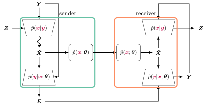
As we have seen, in generative models, expressive power typically comes at the price of ease of inference (and vice versa). So far we have explored three different strategies for this managing trade off: Severely limit expressive power to conjugate or pseudo-conjugate prior distributions in order to allow for exact inference (Chapter 9); allow arbitrarily expressive generative models, but then approximate inference with a separate recogniton model that is arbitrary, but highly parameterized (Sections 10.1 and 10.2), or a generic homogenizer (Section 10.3), or again correct up to simplifying but erroneous independence assumptions (Section 10.4). Now we introduce a fourth strategy: let the latent variables of the model be related to the observed variables by an invertible (and therefore deterministic) transformation. This makes the model marginal ${\hat{p}\mathopen{}\mathclose{{}\left({\color[rgb]{.75,0,.25}\definecolor[named]{pgfstrokecolor}{rgb}{.75,0,.25}\bm{y}}{};\bm{\theta}}\right)}$ computable in closed-form with the standard rules of calculus for changing variables under an integral. Consequently, the marginal relative entropy, $\operatorname*{\text{D}_{\text{KL}}}\mathopen{}\mathclose{{}\left\{{p\mathopen{}\mathclose{{}\left({\bm{Y}}}\right)}\middle\|{\hat{p}\mathopen{}\mathclose{{}\left({\bm{Y}};\bm{\theta}}\right)}}\right\}$, can be descended directly, rather than indirectly via the joint relative entropy, and EM is not needed.

Below we explore two such models in the usual way, starting with simple linear transformations and then moving to more complicated functions. But let us begin with a more abstract formulation, in order to make contact with the unsupervised, discriminative learning problems of Section 7.2. In that section, we related observations ${\bm{\hat{Y}}}$ to (hypothetical) “latent variables” ${\bm{\hat{Z}}}$ via a deterministic, invertible transformation, Eq. 7.23. Here we shall make a similar specification, although to emphasize that this is a generative model, we write the observations as a function of the latent variables, ${\bm{\hat{X}}}$, rather than vice versa. Still, to exhibit the relationship with the discriminative model, we denote this function as the inverse of some “recognition” function, $\bm{d}({\color[rgb]{.75,0,.25}\definecolor[named]{pgfstrokecolor}{rgb}{.75,0,.25}\bm{y}},\bm{\theta})$:

For generative models, it is also necessary to specify a prior distribution over the latent variables. Although the discriminative model makes no such specification, its training objective—maximization of the latent (“output”) entropy—will tend to produce independent outputs. Therefore, we shall assume that the generative model’s latent variables are independent—and, for now, nothing else:

In the second equality, we have simply expressed the probability distributions in terms of the cumulative distribution functions (CDFs), $\psi_{k}({\color[rgb]{.75,0,.25}\definecolor[named]{pgfstrokecolor}{rgb}{.75,0,.25}x_{k}})$, or more precisely their derivatives, in anticipation of the results below.

In the discriminative models of Section 7.2, rather than being specified explicitly, the distribution of latent variables was inherited from the data distribution, ${p\mathopen{}\mathclose{{}\left({\color[rgb]{.75,0,.25}\definecolor[named]{pgfstrokecolor}{rgb}{.75,0,.25}\bm{y}}{}}\right)}$, via the change-of-variables formula. Here something like the reverse obtains: The distribution of the (model) observations ${\hat{p}\mathopen{}\mathclose{{}\left({\color[rgb]{.75,0,.25}\definecolor[named]{pgfstrokecolor}{rgb}{.75,0,.25}\bm{y}}{};\bm{\theta}}\right)}$ is inherited, via the deterministic transformation Eq. 11.1 and the change-of-variables formula, from the distribution of latent variables, Eq. 11.2:

We have recovered Eq. 7.27, but from a different model [5]. Both models use the same map between observations and “latent” variables, given by Eq. 11.1. But the discriminative model proceeds to pass the outputs of this map, $\bm{\check{x}}$, through squashing functions $\bm{\psi}({\color[rgb]{.75,0,.25}\definecolor[named]{pgfstrokecolor}{rgb}{.75,0,.25}\bm{x}})$, whereas the generative model instead interprets $\bm{\psi}({\color[rgb]{.75,0,.25}\definecolor[named]{pgfstrokecolor}{rgb}{.75,0,.25}\bm{x}})$ as the (prior) CDFs of those variables, $\bm{\hat{x}}$. Thus the “outputs” $\bm{\check{z}}$ of the discriminative model are the latent variables of the generative model passed through their own CDFs. If we define $\bm{\hat{z}}\mathrel{\vbox{\hbox{.}\hbox{.} }}=\bm{\psi}(\bm{\hat{x}})$ for the generative model, then we can say that the generative ${\bm{\hat{Z}}}$ are distributed independently (because ${\bm{\hat{X}}}$ are independent and $\bm{\psi}(\cdot)$ acts elementwise) and uniformly (because the CDFs exactly flatten the distribution of ${\bm{\hat{X}}}$). This is consistent with the discriminative objective: maximizing the entropy of ${\bm{\check{Z}}}$ will likewise tend to distribute them independently and uniformly.

Thus, in the deterministic, invertible setting, maximizing mutual information through a discriminative model is equivalent to density estimation in a generative model. It is also useful to re-express the density-estimation problem in terms of ${\bm{\hat{X}}}$:

where ${\check{p}\mathopen{}\mathclose{{}\left({\color[rgb]{.75,0,.25}\definecolor[named]{pgfstrokecolor}{rgb}{.75,0,.25}\bm{x}}{};\bm{\theta}}\right)}$ is the distribution induced by the recognition function applied to the observed data, $\bm{d}({\bm{Y}},\bm{\theta})$. The first equality is Eq. 7.26, and the second can be derived simply by noting that relative entropy is invariant under reparameterization (in this case with $\bm{d}({\color[rgb]{.75,0,.25}\definecolor[named]{pgfstrokecolor}{rgb}{.75,0,.25}\bm{y}},\bm{\theta})$). In light of the second equality, and dropping the language of discriminative and generative models, we can summarize this approach to model fitting like this:

We require a reparameterization of the data, ${\bm{\check{X}}}=\bm{d}({\bm{Y}},\bm{\theta})$, to be distributed close (in the KL sense) to some factorial prior distribution, $\prod_{k=1}^{{K}}\frac{\partial{\psi_{k}}}{\partial{{\color[rgb]{.75,0,.25}\definecolor[named]{pgfstrokecolor}{rgb}{.75,0,.25}\hat{x}_{k}}}}\mathopen{}\mathclose{{}\left({\color[rgb]{.75,0,.25}\definecolor[named]{pgfstrokecolor}{rgb}{.75,0,.25}x_{k}}}\right)$; or, equivalently, to be maximally entropic when “squashed” by $\psi_{k}({\color[rgb]{.75,0,.25}\definecolor[named]{pgfstrokecolor}{rgb}{.75,0,.25}x_{k}})$ (for all $k$).