1.2 What Is a Generative Model?
The core focus of this book is generative models††margin: generative models —but that term has subtly shifted meaning over the last three decades. Still, although it has some other forebears as well, the modern usage is a direct descendant of the original one, and this book traces that descent. In fact, that historical line of development in machine learning provides perhaps the main organizing theme for the entire volume.
1.2.1 Origin (1985)
The Boltzmann machine.
The earliest use of the term “generative model” in machine learning appears to be in Ackley, Hinton, and Sejnowski’s seminal paper describing a learning algorithm for the Boltzmann machine [2]. This is the work that eventually won Geoff Hinton a Nobel Prize. It is appropriate that the chain starts with Hinton, since much of this book develops generative models along the lines he worked out in roughly the period from 1985 – 2010. The authors described the Boltzmann machine as follows:
The network modifies the strengths of its connections so as to construct an internal generative model that produces examples with the same probability distribution as the examples it is shown. (Emphasis in original)
This captures arguably the three essential ingredients that have more or less persisted into the present notion:
-
•
a probabilistic model,
-
•
a training procedure (“modifies the strengths of its connections”), and
-
•
a sampling procedure (“produces examples”).
In particular, the point of the training procedure is to encourage the model to generate samples that are distributed the same way as the training examples.
Latent variables.
In addition, the Boltzmann machine included “hidden” units whose values are not directly constrained by the observed (training) data. The rationale was to allow the network to learn internal representations, under which complicated constraints imposed by the environment on the “visible” units could be expressed, and then satisfied, more simply. But importantly, the hidden units in the Boltzmann machine are not merely deterministic functions of visible units, as in the intermediate layers of a neural network; they are random variables in their own right. Although Ackley did not use this term, they subsequently became known as
-
•
latent variables,
and are also a standard ingredient of many modern generative models. By the mid-90s, Hinton was using “latent-variable” and “generative” as synonymous adjectives.11 1 “What we have just described is an instantiation of the general framework of generative or latent variable models” (emphasis original) [59]. But as we will see, this is perhaps too restrictive a definition for our purposes; for example, it rules out normalizing flows (Chapter 11), in which although there are conceptually two sets of variables, the observed data are merely a deterministic transformation of the hidden variables.
1.2.2 Probabilistic graphical models (1990s)
The concept of the generative model was to shift subtly in the next decade under the impetus of a new synthesis in computer science and statistics. In the late 1980s, Spiegelhalter and Lauritzen [41] unified two seemingly very different computational objects: the so-called Markov random fields that originated in physics to model particle interactions, and had subsequently been generalized by statisticians [17]; and the “belief networks” that Judea Pearl had devised to reason probabilistically about complex systems, like diseases and their symptoms [55]. Spiegelhalter and Lauritzen realized that the two formalisms could be seen as two different kinds of graphical models††margin: probabilistic graphical models (PGMs) , undirected and directed respectively, for which the task of probabilistic inference††margin: probabilistic inference —that is, inferring distributions over some variables, given observations of others—could be solved with a single algorithm (Chapter 5).
Over the next decade, researchers assimilated models from a variety of disciplines into the framework of directed graphical models: hidden Markov models (automatic speech recognition), state-space models (control theory), factor analysis (mathematical psychology), sparse coding (computational neuroscience), and others (Chapter 3; see e.g. [63] and citations therein, and Chapter 10 of [8]). For example, the forward-backward algorithm for the HMMs of the speech-recognition community and the Kalman filter22 2 The smoother of Rausch, Tung, and Striebel, which includes a backward as well as a forward pass, is more properly the counterpart of forward-backward. from control theory turned out to be variations on the same underlying inference algorithm on the same graph, albeit parameterized with different distributions.
The new formalism also encompassed Boltzmann machines, under the framework of undirected graphs. So the canonical generative model could be expressed as a graphical model. More generally, graphical models are inherently probabilistic, admit—at least in theory—both sampling and learning (training) procedures, and explicitly model latent variables. These are the four ingredients I have identified as essential to generative models, so it is no surprise that around this time, they came to be seen as an instance or application of graphical models. And this assimilation was subsequently reinforced by other developments.
1.2.3 Generative and recognition models (1990s)
By the 1990s, the Boltzmann machine had come to be seen as impractical: Its learning algorithm depended on an iterative sampling procedure that only very slowly reaches the equilibrium state in which the samples are valid. This is in part a consequence of allowing each variable to depend directly on all other variables. Interest had therefore shifted towards generative models that assert some form of statistical independence among variables. A particularly appealing structure for generative models is marginal independence between latent variables33 3 In the restricted Boltzmann machine [68], the latent variables are instead conditionally independent. See Section 12.2. and conditional independence between the observed variables, i.e., conditioned on the latent variables. This allows generation to be carried out in two steps: sample the latent variables, and then sample the observed variables (see Fig. 1.1).
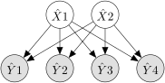
This generation scheme maps nicely onto the intuitive process by which many types of real data are created. For example [59], the process of producing hand-written digits can be schematized as (1) pick a numeral and, say, a writing style (latent variables) and then (2) generate (write) an instance of that numeral (observed variable). Furthermore, inverting the process—that is, computing the probability of a numeral given a hand-written digit—corresponds to probabilistic inference in the corresponding graphical model. This pairing had antecedents in statistics, information theory, and psychology, but under other names, which we turn to next.
The sampling and diagnostic paradigms (1976).
We have implicitly been considering generative models in their role as samplers, but the duality with classifiers furnishes another use. That is, we may be interested in training a generative model purely in order subsequently to invert it and classify data. In this sense, they are the alternatives to fitting a map directly in the other desired direction, from data to labels.
This contrast of approaches to classification dates at least back to the 1970s, but under different names. For example, Efron [15] reviewed the relative merits of logistic regression and linear discriminant analysis (Section 3.1)—in short, the generative approach can be more efficient (fewer samples required to reach the same level of accuracy) if the training data were actually generated by something like the generative model. Dawid considered a more general class of such pairs of classifiers under the heading of the diagnostic and sampling paradigms [7].
In 1995, probably under the influence of the convergence of the neural-networks and statistical literatures under the banner of probabilistic graphical models, Michael Jordan (at that point, still at MIT) filed an influential technical report [34] reviewing these two approaches to classification, using the term generative for the sampling paradigm.44 4 He also suggests as synonyms causal and class-conditional; and for the discriminative approach, diagnostic and predictive. Other terms in the literature for the generative approach to classification include informative [64] and Bayesian. This fixed the terminology for the distinction, so that even today the Wikipedia entry for “generative model” is primarily about generative vs. discriminative classifiers.
Analysis by synthesis (1959).
The idea of constructing generative models to underwrite discrimination had also appeared in an earlier, distinct line of research. Halle and Stevens [20] had argued that the task of recognizing speech—e.g., transformating an acoustic waveform into a sequence of phonemes—was best carried out by first generating waveforms from sequences of phonemes, and then comparing these “hypotheses” to the waveform to be analyzed. They called this analysis by synthesis.55 5 They cite as predecessor to this idea a remarkably prescient reflection from D.M. MacKay on “Mindlike Behaviour in Artefacts” (i.e., machines) [44]. Their own first paper on the topic is from 1959—but it is hard to find! This is extremely similar to Dawid’s “sampling paradigm,” albeit stripped of model fitting and the language of probability and statistics. But the two lines of research do not seem to have been aware of each other at the time.
The influence of analysis by synthesis on the top-down generative models of the 1990s was apparently more or less direct. Its application to the paradigmatic problem of hand-writing recognition [59] appeared as early as 1962, by one of Halle’s colleagues [14]. By the mid-90s, Hinton’s group was citing these papers as predecessors [9]. Interestingly, analysis by synthesis seems to have reached them through the psychology literature66 6 “The old idea of analysis-by-synthesis assumes that the cortex contains a generative model of the world and that recognition involves inverting the generative model in real time.” [9] , which is plausible because it plays a prominent role in Ulric Neisser’s 1967 textbook, Cognitive Psychology [49].
Psychology and neuroscience.
But in some sense the idea is older still. Dayan and colleagues in the aforementioned paper [9] attribute the insight that perception is a form of inference to the 19-century polymath Hermann von Helmholtz. Although not in the language of probability, his Treatise on Physiological Optics [77] argued that visual perception unconsciously brought together incoming sensory information (“sense impressions”) with prior expectations, usually built up through experience, to form the sense of the visual object. He called these “psychic acts of ordinary perception” unconscious inferences.77 7 Although the Southall translation uses “unconscious conclusions.” This is essentially an informal description of Bayes rule,88 8 More precisely, empirical Bayes, since the prior is learned from the data. although Helmholtz did not make this connection. And Bayes rule is the heart of probabilistic inference, i.e. the process by which a top-down generative model is “inverted” so as to compute the probability of the latent variables given the data.
Thus a single framework seemed to encompass an array of quite different technical questions: classification in statistics, computer vision and automatic speech recognition, and even perception in humans and other animals. Artificial neural networks had been intended since the beginning to model fundamental aspects of the nervous system [46], but in the 1990s the top-down generative model seemed to offer the central motif that would unify elements of psychology, probability and statistics, machine vision and audition—and even neuroscience: Whereas feedforward (discriminative) neural networks were the standard approach to (e.g.) image recognition, they are hard to reconcile with the dense feedback and lateral connections found throughout the cerebral cortex.99 9 The axonal projections from primary visual cortex (V1) back to the lateral geniculate nucleus of the thalamus outnumber the forward projections by an order of magnitude. Lateral connections within V1 outnumber feedback connections by another order of magnitude. These are more easily explained in the context of a top-down generative model—or its Bayesian inverse.
Many studies endeavored to make this correspondance more precise, the most influential of which was Olshausen and Field’s famous sparse-coding model (Section 3.1.3, Section 10.1). They showed that a top-down generative model with sparse, independent latent variables—corresponding to the sparse firing of V1 simple cells—, trained to generate patches of natural images, learns to respond most strongly to “Gabor patches”: essentially, localized edges at specific spatial orientations and frequencies. This is remarkable because V1 simple cells prefer precisely the same stimuli. So generative models seemed poised to explain even neurophysiology and neural computation. By the following decade, Hinton was wondering “What kind of a graphical model is the brain?” [26].