|
Lewis, Maryam, and Mike’s Funwork #4 |

|
Brain-State-in-a-Box assignments. |
|
gBSB |
|
The gBSB neural model is a modified form of the BSB model that is better suited for implementing associative memories. The dynamics are defined as
Thus the BSB model can be viewed as a special case of the gBSB model for which the weight matrix W is symmetric and b = 0. One of the useful properties of a gBSB network is the potential to minimize the number of asymptotically stable states that do not correspond to the desired patterns (spurious states). When properly designed, the gBSB network is more effective at minimizing the number of spurious states than the BSB network. In addition to adding the B matrix, the calculation of the W matrix has been modified to reduced the amount of symmetry, and thus further reduce the number of spurious states. For this example, the weight matrix was calculated as
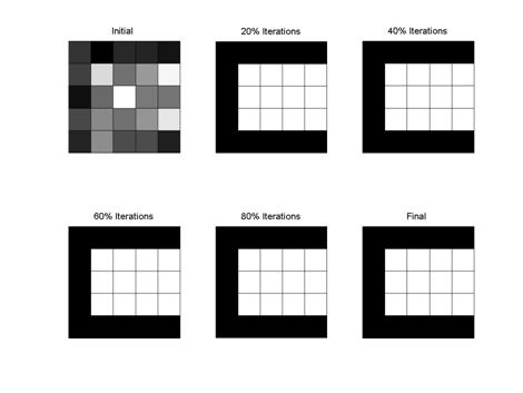
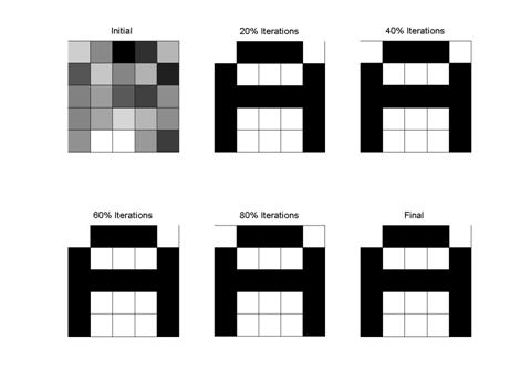
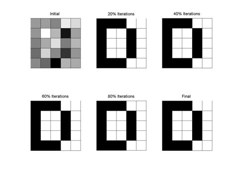
The following figures demonstrate the sample results of a 4-image neural network composed of 25 neurons. The initial images and their progression are shown below. For each run, alpha was set to 0.2 and 20 repetitions were used to arrive at the final value. The noise amplitude maximum was set at ±1.5. The initial and final values of the matrices are also shown for reference. Following the figures is the Matlab code used to perform the analysis. |

|
Matlab Code: function gbsb(reps,alpha,amp) %Create the desired patterns for A, B, C, and D %The letters followed by s indicate the matrix that would be presented to a %a logical display unit. The single letters represent the vectors composed of the %columns of their respective letter matrix stacked together. reps = reps+1; As = [1 -1 -1 -1 1; -1 1 1 1 -1; -1 -1 -1 -1 -1; -1 1 1 1 -1; -1 1 1 1 -1]; Bs = [-1 -1 -1 -1 1; -1 1 1 1 -1; -1 -1 -1 -1 1; -1 1 1 1 -1; -1 -1 -1 -1 1]; Cs = [-1 -1 -1 -1 -1; -1 1 1 1 1; -1 1 1 1 1; -1 1 1 1 1; -1 -1 -1 -1 -1]; Ds = [-1 -1 -1 1 1; -1 1 1 -1 1; -1 1 1 -1 1; -1 1 1 -1 1; -1 -1 -1 1 1]; A = [As(:,1); As(:,2); As(:,3); As(:,4); As(:,5);]; B = [Bs(:,1); Bs(:,2); Bs(:,3); Bs(:,4); Bs(:,5);]; C = [Cs(:,1); Cs(:,2); Cs(:,3); Cs(:,4); Cs(:,5);]; D = [Ds(:,1); Ds(:,2); Ds(:,3); Ds(:,4); Ds(:,5);]; %Now perform the BSB network creation using W = V*V' %Where V = [A B C D] V = [A B C D]; b = rand*A+rand*B+rand*C+rand*D; Bi = [b b b b]; Di = 1.1*eye(25) + 0.01*rand(25); L = -4.5*eye(25); W = (Di*V - Bi)*pinv(V) + L*(eye(25) - V*pinv(V)); %create a noise matrix that is random, but change the distribution so that is is about 0 instead of 0.5 %The constant amp is used to vary the amplitude of the noise vector noise = rand(25,1) - 0.5*ones(25,1); %amp = 2; x = D - amp*noise; %outer loop performs the number of repetitions (i) %inner loop performs the saturation function on each element (j) for i = 2:reps Wx = alpha*(W*x(:,i-1) + b); for j = 1:25 x(j,i) = 0.5*(abs(x(j,i-1) + Wx(j) +1) - abs(x(j,i-1) + Wx(j) -1)); end end initial = [x(1:5,1) x(6:10,1) x(11:15,1) x(16:20,1) x(21:25,1)] final = [x(1:5,reps) x(6:10,reps) x(11:15,reps) x(16:20,reps) x(21:25,reps)] titles = [' Initial '; '20% Iterations'; '40% Iterations'; '60% Iterations'; '80% Iterations'; ' Final ']; sc = (reps-1)/5; for k = 0:5 subplot(2,3,(k+1)) col = ceil(sc*k + 1); if ((col)<=reps) X = [x(1:5,(col)) x(6:10,(col)) x(11:15,(col)) x(16:20,(col)) x(21:25,(col))]; ABCD(X) title(titles(k+1,:)) end end |
|
Figure A. Depiction of the convergence of the distorted image of A into the original image stored. initial = 1.1225 -0.0345 -2.3307 -1.4953 0.6979 -0.9012 1.0022 -0.0953 0.6658 -1.7559 -0.1554 0.3326 -0.8052 -1.2497 0.0765 -0.1144 0.4339 1.2478 0.7351 0.0512 0.1537 1.9168 1.9676 0.2703 -1.3113 final = 1.0000 -1.0000 -1.0000 -1.0000 1.0000 -1.0000 1.0000 1.0000 1.0000 -1.0000 -1.0000 -1.0000 -1.0000 -1.0000 -1.0000 -1.0000 1.0000 1.0000 1.0000 -1.0000 -1.0000 1.0000 1.0000 1.0000 -1.0000 |
|
Figure B. Depiction of the convergence of the distorted image of B into the original image stored. initial = -1.7855 -1.3547 -0.7903 0.4747 0.3443 0.1233 2.1170 0.6643 -0.0880 -2.3359 -0.1725 -0.3332 -0.7011 -0.3406 0.6812 0.1305 2.3434 0.8684 2.2642 0.3751 0.3194 -0.7908 -0.6074 -0.0478 0.5738 final = -1.0000 -1.0000 -1.0000 -1.0000 1.0000 -1.0000 1.0000 1.0000 1.0000 -1.0000 -1.0000 -1.0000 -1.0000 -1.0000 1.0000 -1.0000 1.0000 1.0000 1.0000 -1.0000 -1.0000 -1.0000 -1.0000 -1.0000 1.0000 |
|
Figure C. Depiction of the convergence of the distorted image of C into the original image stored. initial = -1.3489 -2.3562 -1.6189 -1.6678 -1.9740 -1.1506 1.6195 -0.3102 0.4278 2.0985 -2.0649 -0.4625 2.3026 -0.1208 -0.2195 -1.0426 0.1348 -0.2976 0.3816 1.8418 -1.6512 0.2324 -0.9305 -0.9695 -1.7160 final = -1.0000 -1.0000 -1.0000 -1.0000 -1.0000 -1.0000 1.0000 1.0000 1.0000 1.0000 -1.0000 1.0000 1.0000 1.0000 1.0000 -1.0000 1.0000 1.0000 1.0000 1.0000 -1.0000 -1.0000 -1.0000 -1.0000 -1.0000 |
|
Figure D. Depiction of the convergence of the distorted image of D into the original image stored. initial = 0.1939 0.2781 -0.1173 1.5602 1.3352 0.1283 1.9668 0.7142 -2.0544 0.3522 -0.1893 0.5052 1.3996 -0.2558 0.6769 -0.5124 1.1892 -0.0187 -1.5052 0.1418 -0.0517 -0.5908 -2.3987 0.6305 0.5303 final = -1.0000 -1.0000 -1.0000 1.0000 1.0000 -1.0000 1.0000 1.0000 -1.0000 1.0000 -1.0000 1.0000 1.0000 -1.0000 1.0000 -1.0000 1.0000 1.0000 -1.0000 1.0000 -1.0000 -1.0000 -1.0000 1.0000 1.0000 |