|
WTA & Hopfield Net Demonstrations
by Andy Byerly & Ricky Chan
WINNER TAKES ALL ALGORITHM
MATLAB CODE
You may download the Matlab code here.
function w = wta(x, w)
% WTA - Winner Takes All training algorithm
%
% INPUT
% x - training patterns
% w - initial weight
%
% OUTPUT
% w - updated weight
%
% Andy Byerly
% Ricky Chan
% ECE 595C
% October 9, 2004
alpha = 0.5;
% If there's no input specified, these parameters will be utilized
if nargin ~= 2
x = [-1 0 1/sqrt(2);
0 1 1/sqrt(2)];
w = [ 0 -2/sqrt(5) -1/sqrt(5);
-1 1/sqrt(5) 2/sqrt(5)];
end
[rowx, colx] = size(x);
[roww, colw] = size(w);
maxResult = 0;
maxIndex = 0;
figure(1)
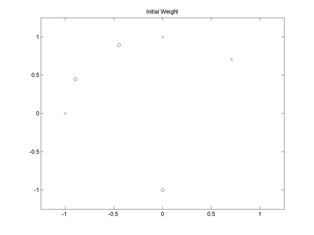
plot(x(1,:), x(2,:), 'rx', w(1,:), w(2,:), 'bo')
title('Initial Weight')
axis([-max(max(abs(x)))-.25 max(max(abs(x)))+.25 -max(max(abs(x)))-.25 max(max(abs(x)))+.25])
% Looking for the index of the winning weight
for counter = 1:colx
x(:,counter) = x(:,counter)/norm(x(:,counter));
for counter2 = 1:colw
w(:,counter2) = w(:,counter2)/norm(w(:,counter2));
dotProduct = dot(w(:,counter2),x(:,counter));
if dotProduct > maxResult
maxResult = dotProduct;
maxIndex = counter2;
end
end
% Updating the winning weight
w(:,maxIndex) = w(:,maxIndex) + alpha*(x(:,counter) - w(:,maxIndex));
% Scaling it to have a unit length
w(:,maxIndex) = w(:,maxIndex)/norm(w(:,maxIndex));
end
% Plotting the result,
figure(2)
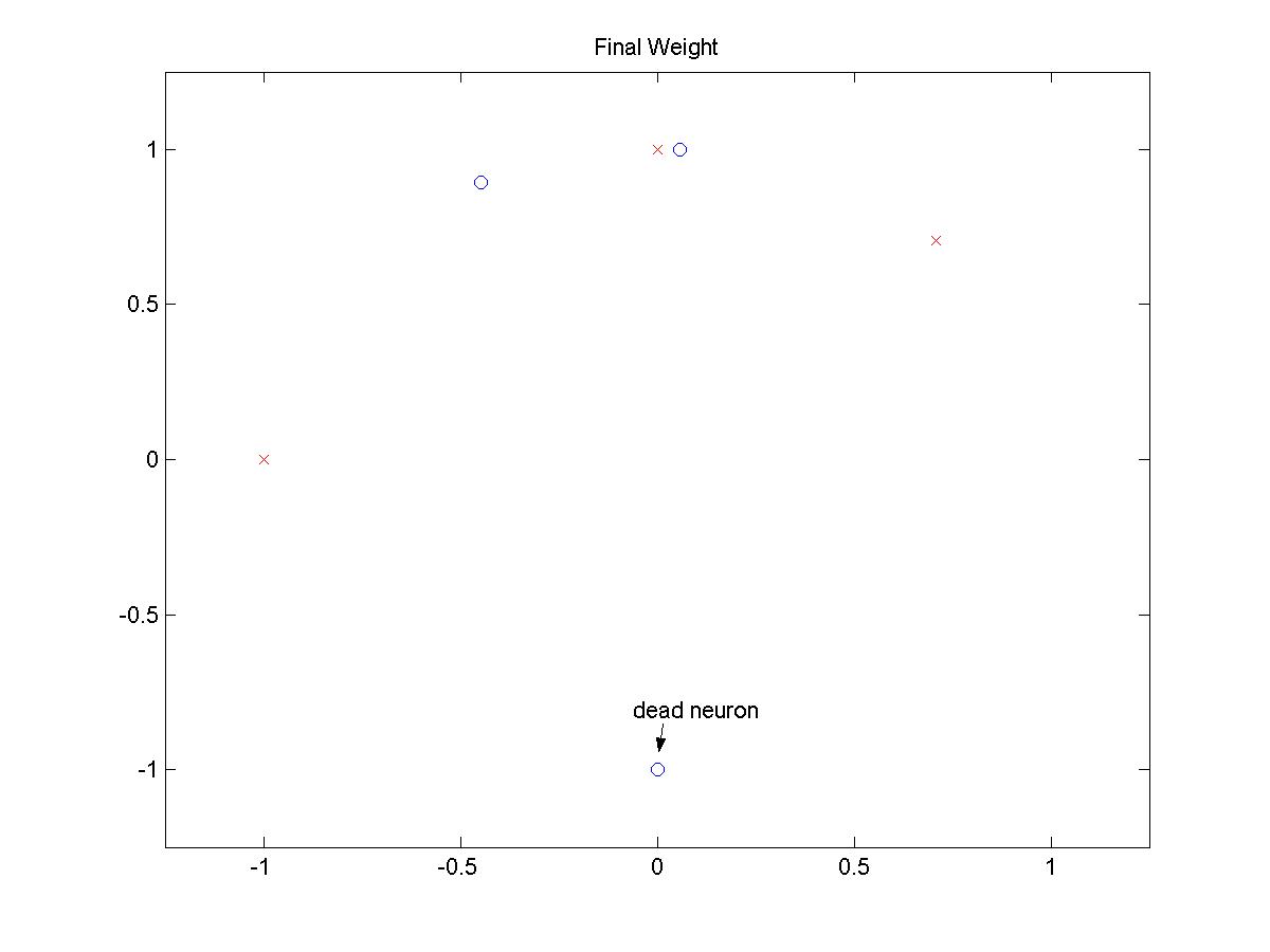
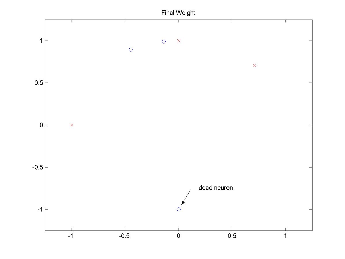
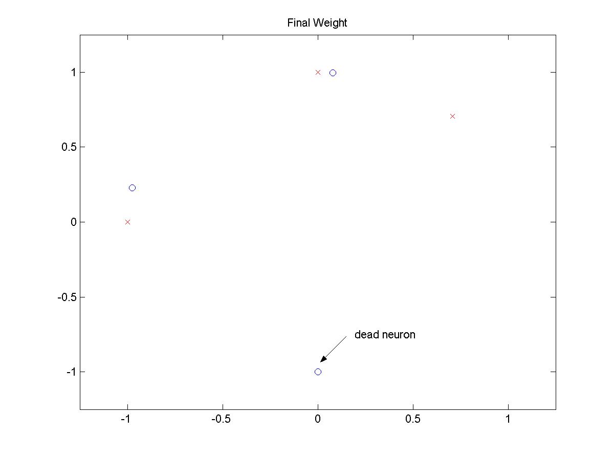
plot(x(1,:), x(2,:), 'rx', w(1,:), w(2,:), 'bo')
axis([-max(max(abs(x)))-.25 max(max(abs(x)))+.25 -max(max(abs(x)))-.25 max(max(abs(x)))+.25])
RESULTS
Pattern 1:

INITIAL POSITIONS
 (click on image to open larger picture)
|
FINAL POSITIONS
 (click on image to open larger picture)
|
Pattern 2:

INITIAL POSITIONS
 (click on image to open larger picture)
|
FINAL POSITIONS
 (click on image to open larger picture)
|
Pattern 3:

INITIAL POSITIONS
 (click on image to open larger picture)
|
FINAL POSITIONS
 (click on image to open larger picture)
|
From exhaustive experiment with different patterns, it is concluded that there is no
input sequences that does not create a dead neuron.
HOPFIELD NETWORK ALGORITHM
PROBLEM STATEMENT
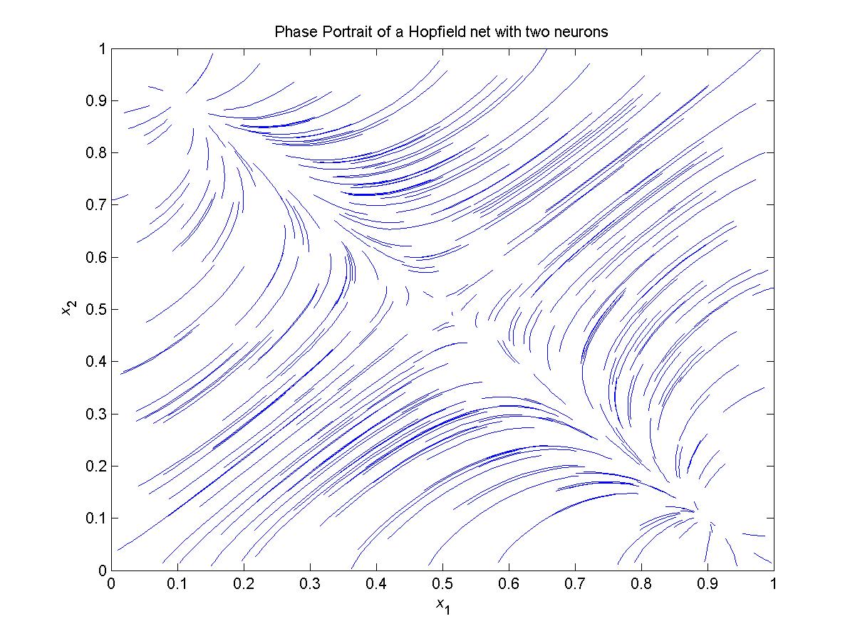
Construct a Hopfield net with two neurons and generate its phase portrait.
Matrix representation of the circuit realization of the Hopfield net:

Need to determine different values for R11, R12, R22, r1, and r2.
Two equilibrium points are chosen (0.1, 0.9) and (0.9, 0.1)
and GA (Genetic Algorithm) is utilized to solve the parameter values.
The fitness function of the GA minimizes the gradient of the (Cost)Error function,
shown as follows:

The result from the GA shows the parameters as follows:

You may download the GA functions here.
MATLAB CODE
You may download the Matlab code here.

function hopfield(C, R, I)

% HOPFIELD -   Hopfield network with two neurons
%
% CALL ROUTINE
%   hopfield(C, R, I)
%
% INPUT
%   C      -   Capacitance vector
%              [C1 C2]
%   R      -   Resistance matrix
%              [R11 R12]
%              [R12 R22]
%   I      -   External input vector
%              [I1 I2]
%
% OUTPUT
%   This function will produce the phase portrait of the Hopfield neural
%   nets
%
% Andy Byerly
% Ricky Chan
% ECE 595C
% October 9, 2004


close all;
clc


% If there's no input specified, these parameters will be utilized
if nargin ~= 3
    C = [1 1];
    R = [12.8272 -12.8375;
         -12.8375 12.7193];
    r = [34.8009 35.3497];
    I = [0 0];
end

global R11 R12 R21 R22 C1 C2 r1 r2 I1 I2 theta
theta = 1;
R11 = R(1,1);
R12 = R(1,2);
R21 = R(2,1);
R22 = R(2,2);
C1 = C(1);
C2 = C(2);
r1 = r(1);
r2 = r(2);
I1 = I(1);
I2 = I(2);
tspan=[0 20];
numIter = 300;
max = 1-eps;
min = eps;
rand('state',sum(100*clock));

figure
for counter = 1:numIter
    x0 = rand(2,1)*(max-min) + min;
    x0 = x0';
    [t,x]=ode23s('plant',tspan,x0);
    plot(x(:,1),x(:,2));
    hold on
end

axis([0 1 0 1]);
title('Phase Portrait of a Hopfield net with two neurons');
xlabel('{\it x}_1');
ylabel('{\it x}_2');

function u = sigInv(x, theta)

% SIGINV    - Inverse of Sigmoid function
%
% CALL ROUTINE
%   u = sigInv(x, theta)
%
% INPUT
%   x       -   vector output of the nonlinear amplifier
%   theta   -   slope of the Sigmoid function
%
% OUTPUT
%   u       -   input to the nonlinear amplifier

u = theta.*(log(x) - log(1-x));

function y = dsigInvdx(x, theta)

% DSIGINVDX    - derivative of the Inverse of Sigmoid function
%
% CALL ROUTINE
%   u = dsigInvdx(x, theta)
%
% INPUT
%   x       -   vector output of the nonlinear amplifier
%   theta   -   slope of the Sigmoid function
%
% OUTPUT
%   u       -   input to the nonlinear amplifier

y = theta.*(1./x + 1./(1-x));


ADDITIONAL MATLAB FUNCTIONS
You may download the Matlab code here.

function xdot=plant(t,x);

% PLANT -   function to be used with ode23s
%
% INPUT
%   t   -   time vector according to the time span specified
%   x   -   values of x to be simulated
%
% OUTPUT
%   xdot    -   time derivative of the plant

global R11 R12 R21 R22 C1 C2 r1 r2 I1 I2 theta
xdot =[((x(1)/R11) + (x(2)/R12) + I1 - (sigInv(x(1), theta)/r1))./(C1.*dsigInvdx(x(1), theta));
       ((x(1)/R21) + (x(2)/R22) + I2 - (sigInv(x(2), theta)/r2))./(C2.*dsigInvdx(x(1), theta))];

function u = sigInv(x, theta)

% SIGINV    - Inverse of Sigmoid function
%
% CALL ROUTINE
%   u = sigInv(x, theta)
%
% INPUT
%   x       -   vector output of the nonlinear amplifier
%   theta   -   slope of the Sigmoid function
%
% OUTPUT
%   u       -   input to the nonlinear amplifier
u = theta*(log(x) - log(1-x));

function y = dsigInvdx(x, theta)

% DSIGINVDX    - derivative of the Inverse of Sigmoid function
%
% CALL ROUTINE
%   u = dsigInvdx(x, theta)
%
% INPUT
%   x       -   vector output of the nonlinear amplifier
%   theta   -   slope of the Sigmoid function
%
% OUTPUT
%   u       -   input to the nonlinear amplifier

y = (theta./x) + theta./(1-x);
RESULTS
 (click on image to open larger picture)
Due to the chosen technique that chooses the equilibrium points to be
located at (0.1, 0.9) and (0.9, 0.1), one may clearly conclude from the figure
that those are the two equilibrium points.
|