|
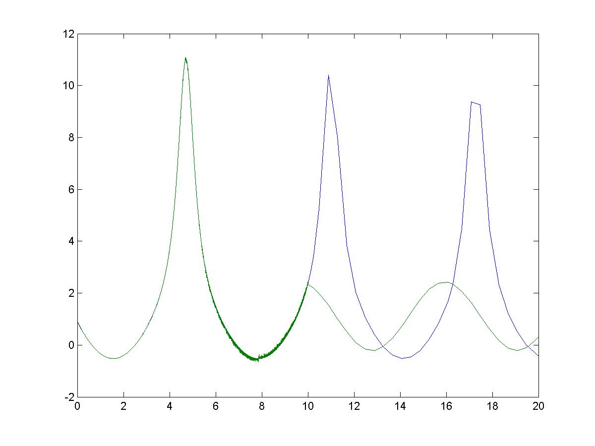
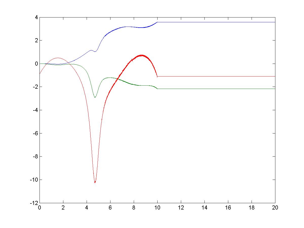
OFFLINE ADALINE LEARNING OFFLINE ADALINE LEARNINGThe offline Adaline Learning algorithm utilizes an adaptive algorithm to minimize error between the output of the plant and the desired output. The weight vectors are determined by the adaptive algorithm and are held constant at t = 10 secs. The plots are shown below. One will observe that the constant weight vectors do not maintain zero error. As the diagrams below suggest, the following simulation was completed in Simulink. The Simulink file is available here: adaline.mdl SYSTEM
EQUATIONS 
RESULTS
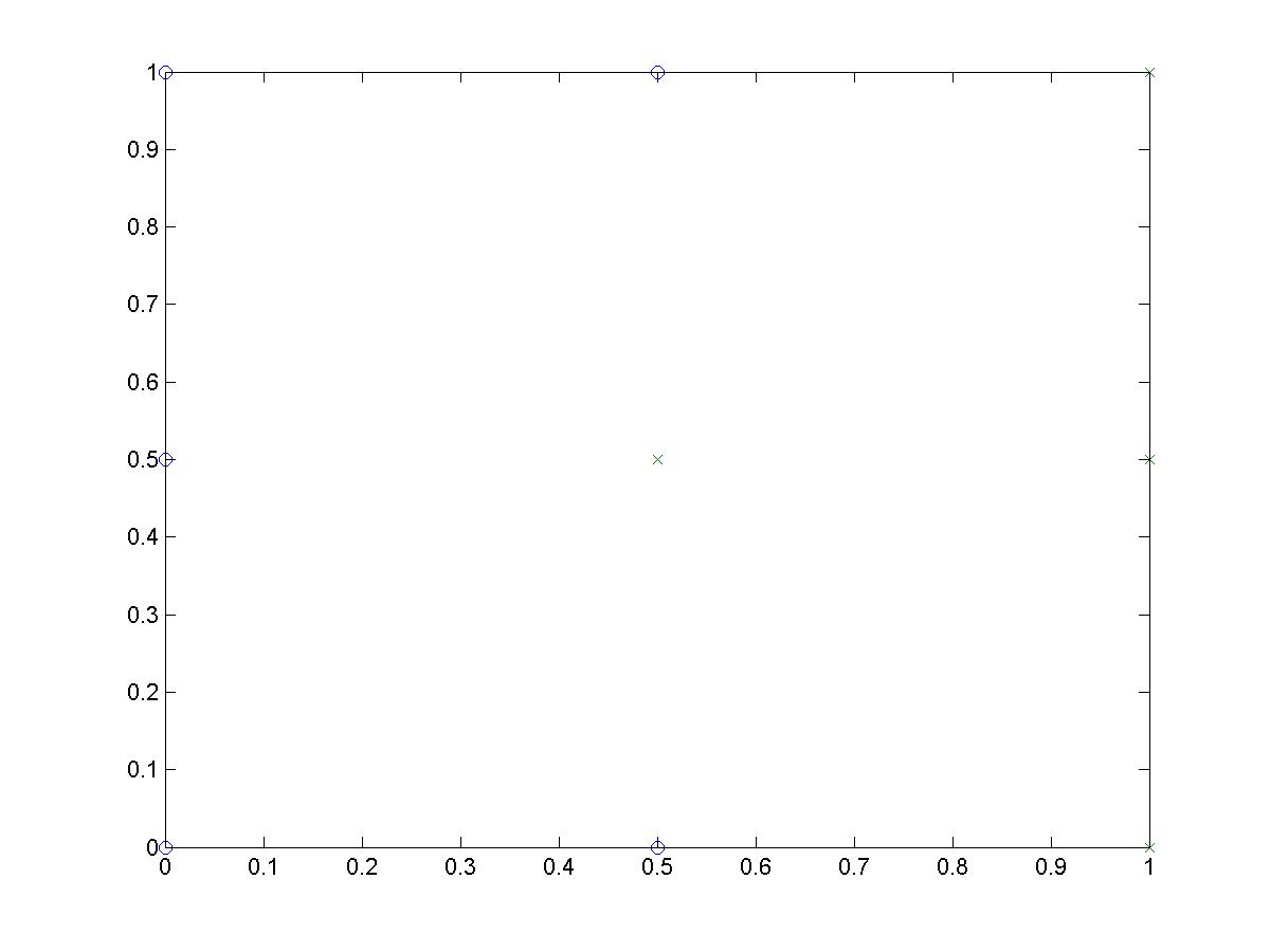
TWO LAYER PERCEPTION IMPLEMENTATIONThe two layer perceptron intends to seperate non-linearly seperable sets that could not be solved using TLUs. This example seperates the problem shown below. The code shown below could be used to solve other non-linearly seperable problems. The code may also be adapted to include even higher layers of perceptrons. The following simulation was performed in Matlab. The Matlab file is available here: perceptron.m MATLAB CODEfunction [W,dActual] = perceptron(x,d)
alpha = 0.75;
N = 50000;
W = rand(3,3);
for counter = 1:N
index = mod(counter-1,size(x,2))+1;
[y,z] = evaluatePerceptron(W,x(:,index));
gradientE = zeros(3,3);
for i = 1:2
for j = 1:3
gradientE(j,i) = -(d(index)-y)*y*(1-y)*W(i,3)*z(i)*(1-z(i))*x(j,index);
end
end
for j = 1:3
gradientE(j,3) = -(d(index)-y)*y*(1-y)*z(j);
end
W = W-alpha*gradientE;
end
dactual = zeros(size(d));
for counter = 1:size(x,2)
dActual(counter) = evaluatePerceptron(W,x(:,counter));
end
X = 0:0.01:1;
Y = X;
Z = zeros(length(Y),length(X));
for i = 1:length(X)
for j = 1:length(Y)
Z(j,i) = evaluatePerceptron(W,[X(i);Y(j);-1]);
end
end
mesh(X,Y,Z);
view(-10,35);
return
function f = sigmoid(v)
f = 1/(1+exp(-v));
return
function [y,z] = evaluatePerceptron(W,x)
z = [sigmoid(W(:,1)'*x);sigmoid(W(:,2)'*x);-1];
y = sigmoid(W(:,3)'*z);
return
MATLAB FUNCTION CALL >> [W,d] = perceptron([0,0,0,0.5,0.5,0.5,1,1,1;0,0.5,1,0,0.5,1,0,0.5,1;
-1,-1,-1,-1,-1,-1,-1,-1,-1],[0,0,0,0,1,0,1,1,1])
W =
9.4400 7.4031 6.4046
-8.4903 6.7129 6.9753
-1.7083 5.1559 9.7832
d =
0.0131 0.0002 0.0177 0.1122 0.8852 0.1070 0.9493 0.9725 0.9599
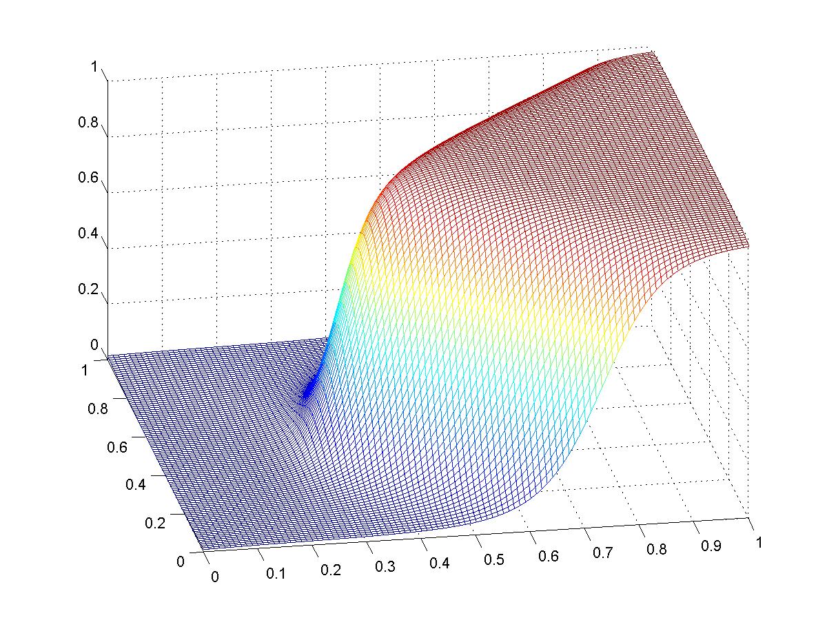
TWO LAYER PERCEPTRON MESH RESULTS
|
||||||||||||
|
Please refer to the following text for further information regarding the above two algorithms: Stanislaw H. Żak, Systems and Control, Oxford University Press, New York, 2003, ISBN 0-19-515011-2 |
||||||||||||