This appeared as an invited paper presented at the ATR Workshop on "A Biological Framework for Speech Perception and Production," September 16-17, 1994, Kyoto Japan. This HTML version of the technical report differs from the paper copy by including the sound reconstructions.
Some of this work was performed by Malcolm Slaney, Daniel Naar and Richard F. Lyon while all three were employed at Apple Computer. The mathematical details of this work were presented at the 1994 ICASSP [1].
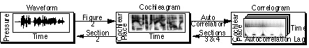
Figure 1. Three stages in low-level auditory perception are shown here. Sound waves are converted into a detailed representation with broad spectral bands, known as cochleagrams. The correlogram then summarizes the periodicities in the cochleagram with short-time autocorrelation. The result is a perceptual movie synchronized to the acoustic signal. The two inversion problems addressed in this work are indicated with arrows from right to left.
The inversion techniques described here are important because they allow us to readily evaluate the results of sound separation models that "zero out" unwanted portions of the signal in the correlogram domain. This work extends the convex projection approach of Irino [5] and Yang [6] by considering a different cochlear model, and by including the correlogram inversion. The convex projection approach is well suited to "filling in" missing information. While this paper only describes the process for one particular auditory model, the techniques are equally useful for other models.
This paper describes three aspects of the problem: cochleagram inversion, conversion of the correlogram into spectrograms, and spectrogram inversion. A number of reconstruction options are explored in this paper. Some are fast, while other techniques use time-consuming iterations to produce reconstructions perceptually equivalent to the original sound. Fast versions of these algorithms could allow us to separate a speaker's voice from the background noise in real time.

Figure 2. Three stages of the simple cochlear model used in this paper are shown above.
The cochleagram is converted back into sound by reversing the three steps shown in Figure 2. First the AGC is divided out, then the negative portions of each cochlear channel are recovered by using the fact that each channel is spectrally limited. Finally, the cochlear filters are inverted by running the filters backwards, and then correcting the resulting spectral slope.
The AGC stage in this cochlear model is controlled by its own output. It is a combination of a multiplicative gain and a simple first-order filter to track the history of the output signal. Since the controlling signal is directly available, the AGC can be inverted by tracking the output history and then dividing instead of multiplying. The performance of this algorithm is described by Naar [8] and will not be addressed here. It is worth noting that AGC inversion becomes more difficult as the level of the input signal is raised, resulting in more compression in the forward path.
The next stage in the inversion process can be done in one of two ways. After AGC inversion, both the positive values of the signal and the spectral extant of the signal are known. Projections onto convex sets [9], in this case defined by the positive values of the detector output and the spectral extant of the cochlear filters, can be used to find the original signal. This is shown in the left half of Figure 3. Alternatively, the spectral projection filter can be combined with the next stage of processing to make the algorithm more efficient. The increased efficiency is due to better match between the spectral projection and the cochlear filterbank, and due to the simplified computations within each iteration. This is shown in the right half of Figure 3. The result is an algorithm that produces nearly perfect results with no iterations at all.
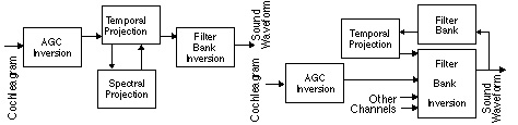
Figure 3. There are two ways to use convex projections to recover the information lost by the detectors. The conventional approach is shown on the left. The right figure shows a more efficient approach where the spectral projection has been combined with the filterbank inversion
Finally, the multiple outputs from the cochlear filterbank are converted back into a single waveform by correcting the phase and summing all channels. In the ideal case, each cochlear channel contains a unique portion of the spectral energy, but with a bit of phase delay and amplitude change. For example, if we run the signal through the same filter the spectral content does not change much but both the phase delay and amplitude change will be doubled. More interestingly, if we run the signal through the filter backwards, the forward and backward phase changes cancel out. After this phase correction, we can sum all channels and get back the original waveform, with a bit of spectral coloration. The spectral coloration or tilt can be fixed with a simple filter. A more efficient approach to correct the spectral tilt is to scale each channel by an appropriate weight before summing, as shown in Figure 4. The result is a perfect reconstruction, over those frequencies where the cochlear filters are non-zero.

Figure 4. Two approaches are shown here to invert the filterbank. The left diagram shows the normal approach, the right figure shows a more efficient approach where the spectral-tilt filter is converted to a simple multiplication.
Figure 5 shows results from the cochleagram inversion procedure. An impulse is shown on the left, before and after 10 iterations of the HWR inversion (using the algorithm on the right half of Figure 3). With no iterations the result is nearly perfect, except for a bit of noise near the center. The overall curvature of the baseline is due to the fact that information near DC has been lost as it travels through the auditory system and there is no way to recover it with the information that we have. A more interesting example is shown on the right. Here the word "tap" has been reconstructed, with and without the AGC inversion. With the AGC inversion the result is nearly identical to the original. The auditory system is very sensitive to onsets and quickly adapts to steady state sounds like vowels. It is interesting to compare this to the reconstruction without AGC inversion. Without the AGC, the result is similar to what the ear hears, the onsets are more prominent and the vowels are deemphasized. This is shown in the right half of Figure 5.
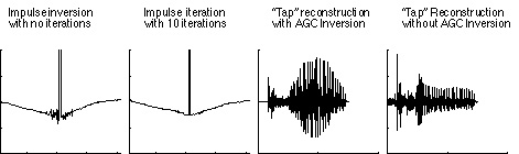
Figure 5. The cochlear reconstructions of an impulse and the word "tap" are shown here. The first and second reconstructions show an impulse reconstruction with and without iterations. The third and fourth waveforms are the word "tap" with and without the AGC inversion.This sound example is the original utterance used in all of these studies (play tapestry.aiff example).
This sound example is the cochlear reconstruction of the "tapestry" sample with 10 iterations through the cochlear model inversion loop (play CochInvTenIterations.aiff example).
This sound example is the reconstruction of a low level signal with the AGC inversion turned off (play CochInvNoAGCLow.aiff example).
This sound example is the reconstruction of a high level signal with the AGC inversion turned off. Note the resulting signal is highly compressed compared to the low-level signal and especially to the original utterance (play CochInvNoAGCHigh.aiff example).
But through all these changes in the cochlear filters, the timing information in the signal is preserved. The spectral profile, as measured by the cochlea, might change, but the rate of glottal pulses is preserved. Thus I believe the auditory system is based on a representation of sound that makes short-time periodicities apparent. One such representation is the correlogram. The correlogram measures the temporal correlation within each channel, either using FFTs which are most efficient in computer implementations, or neural delay lines much like those found in the binaural system of the owl.
The process of inverting the correlogram is simplified by noting that each autocorrelation is related by the Fourier transform to a power spectrum. By combining many power spectrums into a picture, the result is a spectrogram. This process is shown in Figure 6. In this way, a separate spectrogram is created for each channel. There are known techniques for converting a spectrogram, which has amplitude information but no phase information, back into the original waveform. The process of converting from a spectrogram back into a waveform is described in Section 4. The correlogram inversion process consists of inverting many spectrograms to form an estimate of a cochleagram. The cochleagram is inverted using the techniques described in Section 2.
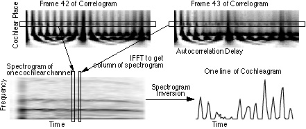
Figure 6. Correlogram inversion is possible by noting that each row of the correlogram contains the same information as a spectrogram of the same row of cochleagram output. By converting the correlogram into many spectrograms, the spectrogram inversion techniques described in Section 4 can be used. The lower horizontal stripe in the spectrogram is due to the narrow passband of the cochlear channel. Half-wave rectification of the cochlear filter output causes the upper horizontal stripes.
One important improvement to the basic method is possible due to the special characteristics of the correlogram. The essence of the spectrogram inversion problem is to recover the phase information that has been thrown away. This is an iterative procedure and would be costly if it had to be performed on each channel. Fortunately,there is quite a bit of overlap between cochlear channels. Thus the phase recovered from one channel can be used to initialize the spectrogram inversion for the next channel. A difficulty with spectrogram inversion is that the absolute phase is lost. By using the phase from one channel to initialize the next, a more consistent set of cochlear channel outputs is recovered.
The basic procedure in spectrogram inversion [10] consists of iterating between the time and the frequency domains. Starting from the frequency domain, the magnitude but not the phase is known. As an initial guess, any phase value can be used. The individual power spectra are inverse Fourier transformed and then summed to arrive at a single waveform. If the original spectrogram used overlapping windows of data, the information from adjacent windows either constructively or destructively interferes to estimate a waveform. A spectrogram of this new data is calculated, and the phase is now retained. We know the original magnitude was correct. Thus we can estimate a better spectrogram by combining the original magnitude information with the new phase information. It can be shown that each iteration will reduce the error.
Figure 7 shows an outline of steps that can be used to improve the consistency of phase estimates during the first iteration. As each portion of the waveform is added to the estimated signal, it is possible to add a linear phase so that each waveform lines up with the proceedings segments. The algorithm described in the paragraph above assumes an initial phase of zero. A more likely phase guess is to choose a phase that is consistent with the existing data. The result with no iterations is a waveform that is often closer to the original than that calculated assuming zero initial phase and ten iterations.
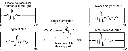
Figure 7. A procedure for adjusting the phase of new segments when inverting a spectrogram is shown above. As each new segment (bottom left) is converted from a power spectrum into a waveform, a linear phase is added to maximize the fit with the existing segments (top left.) The amount of rotation is determined by a cross correlation (middle). Adding the new segment with the proper rotation (top right) produces the new waveform (bottom right.)The four sound examples here show the effect of spectrogram inversion, with and without the phase prediction algorithm shown in Figure 7, and with and without a number of iterations.
Zero Iterations and zero phase guess at each frame. The flat pitch is due to the frame rate of the spectrogram calculation (play SpecInvZeroPhase0.aiff example).
Ten iterations starting with zero phase. The result isn't very good yet (play SpecInvZeroPhase10.aiff example).
But now let's use the phase prediction algorithm. This result, even with no iterations sounds better then the reconstruction with 10 iterations and no phase guess (play SpecInvRotatedPhase0.aiff example).
Finally, with rotated phase , there isn't much room for improvement. Here is the result with ten iterations (play SpecInvRotatedPhase10.aiff example).
The total computational cost is minimized by combining these improvements with the initial phase estimates from adjacent channels of the correlogram. Thus when inverting the first channel of the correlogram, a cross-correlation is used to pick the initial phase and a few more iterations insure a consistent result. After the first channel, the phase of the proceeding channel is used to initialize the spectrogram inversion and only a few iterations are necessary to fine tune the waveform.
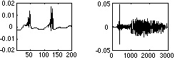
Figure 8. Reconstructions from the correlogram representation of an impulse train and the word "tap" are shown above. Reducing the input signal level, thus minimizing the effect of errors when inverting the AGC, produces results identical to the original "tap."It is important to note that the algorithms described in this paper are designed to minimize the error in the mean-square sense. This is a convenient mathematical definition, but it doesn't always correlate with human perception. A trivial example of this is possible by comparing a waveform and a copy of the waveform delayed by 10ms. Using the mean-squared error, the numerical error is very high yet the two waveforms are perceptually equivalent. Despite this, the results of these algorithms based on mean-square error do sound good.This sound example is the result of inverting a correlogram and using no iterations when converting from the autocorrelations to cochlear waveforms (play CorInvZeroIter.aiff) example. The only error I can hear is the /u/ in hung sounds funny.
This second example shows the result of a correlogram inversion with ten iterations. The original reconstruction sounded pretty good, so there isn't much difference (play CorInvZeroIter.aiff example).
These techniques will be especially useful as part of a sound separation system. I do not believe that our auditory system resynthesizes partial waveforms from the auditory scene. Yet, all systems generate separated sounds so that we can more easily perceive their success. More work is still needed to fine-tune these algorithm and to investigate the ability to reconstruct sounds from partial correlograms.
This work in this paper was performed with Daniel Naar and Richard F. Lyon. We are grateful for the help we have received from Richard Duda (San Jose State), Shihab Shamma (U. of Maryland), Jim Boyles (The MathWorks) and Michele Covell (Interval Research).
[2] M. Slaney and R. F. Lyon, "On the importance of time-A temporal representation of sound," in Visual Representations of Speech Signals, eds. M. Cooke, S. Beet, and M. Crawford, J. Wiley and Sons, Sussex, England, 1993.
[3] R. F. Lyon, "A computational model of binaural localization and separation," Proc. of IEEE ICASSP, 1148-1151, 1983.
[4] M. Weintraub, "The GRASP sound separation system," Proc. of IEEE ICASSP, pp. 18A.6.1-18A.6.4, 1984.
[5] T. Irino, H. Kawahara, "Signal reconstruction from modified auditory wavelet transform," IEEE Trans. on Signal Processing, 41, 3549-3554, Dec. 1993.
[6] X. Yang, K. Wang, and S. Shamma, "Auditory representations of acoustic signals," IEEE Trans. on Information Theory, 38, 824-839, 1992.
[7] R. F. Lyon, "A computational model of filtering, detection, and compression in the cochlea," Proc. of the IEEE ICASSP, 1282-1285, 1982.
[8] D. Naar, "Sound resynthesis from a correlogram," San Jose State University, Department of Electrical Engineering, Technical Report #3, May 1993.
[9] R. W. Papoulis, "A new algorithm in spectral analysis and band-limited extrapolation," IEEE Trans. Circuits Sys., vol. 22, 735, 1975.
[10] D. Griffin and J. Lim, "Signal estimation from modified short-time Fourier transform," IEEE Trans. on Acoustics, Speech, and Signal Processing, 32, 236-242, 1984.
[11] F. S. Cooper, "Some Instrumental Aids to Research on Speech," Report on the Fourth Annual Round Table Meeting on Linguistics and Language Teaching, Georgetown University Press, 46-53, 1953.
[12] F. S. Cooper, "Acoustics in human communications: Evolving ideas about the nature of speech," J. Acoust. Soc. Am., 68(1), 18-21, July 1980.