Week 4 - LP Applications with LINDO

Assignment:

Review this document.

Read sections 1.1-1.9 in the text "Expert Systems: Principles and Programming."

Use the LINDO LP solver software to solve the following problems. Problems are due Friday of week 5 at class time.

60 points

1. You own a company that provides a service that is required 7 days per week. Your employees are entitled to 2 consecutive days off per week. You have estimated the number of employees required per work day based on data from previous operation of the company as shown in the table below.

                   Mon    Tue   Wed   Thu  Fri  Sat  Sun  
   No. Employees    18     16    15    16   19   14   12
   

   Find the number of employees to schedule to start a five-day stint on each day of the week (use an LP formulation). Note: Be sure to look at the example staff covering problem.

2. A fertilizer manufacturer has just received a contract to supply 10,000 tons of 3-12-12 fertilizer. The guaranteed composition of this fertilizer is (by weight) at least 3% nitrogen, 12% phosphorus and 12% potash. The fertilizer can be mixed from any combination of the raw materials described in the table below.

                                                      Current
   Raw Material  % Nitrogen  % Phosphorus  % Potash   World
                                                     Price/Ton
   
      AN            50             0          0        $19
      SP             1            40          5         18
      CP             2             4         35         17.50
      BG             1            15         17         21.50
   

   The fertilizer company also has an option to purchase 3-12-12 fertilizer from another company at $19.50/ton. Assuming the cost of mixing and transportation is zero, should the company buy fertilizer from the second company or mix their own? If the company should mix their own fertilizer, what is the proportion of each ingredient?

   See the example blending problem for additional help in formulating this type of problem.

3. A farmer has four fields (F1, F2, F3, and F4) and two sites (S1 and S2) at which grain from these four fields can be stored. Storage site S1 can store a maximum of 725 cubic meters of grain and site S2 can store a maximum of 555 cubic meters of grain. The distances between fields and storage sites are given below.

                 Total          Distance to
   Field     Yield (m**3)       S1       S2
   F1            155            27 km    11 km
   F2            282            13       29
   F3            261            13       10
   F4            455            26       10
   

   Grain will be transported from the fields to the storage locations with a truck that has a capacity of 10 cubic meters. The cost of operating the truck $2.10 per load per kilometer. Find the minimum transportation costs for getting all of the grain from the fields to the storage sites. Also determine the amount of grain from each field that will be hauled to each storage site.

   Note: Be sure to look at the example network problem.

4. A farmer has 120 acres which can be used to produce wheat or corn. The yield is 55 bushels per acre per year for wheat and 95 bushels per acre per year for corn. Labor requirements are 4 hours per acre per years, plus 0.15 hours per bushel of wheat and 0.70 hours per bushel of corn. Cost of seed, fertilizer and other expenses are $.22 per bushel of wheat produced and $.14 per bushel of corn produced. Wheat can be sold for $3.50 per bushel and corn for $2.35 per bushel. Wheat can be purchased for $3.58 per bushel and corn for $2.41 per bushel.

   In addition to corn and wheat, the farmer may raise hogs and/or chickens. The farmer sells both hogs and chickens after they reach 1 year in age (simplifying assumption). A pig sells for $100 and a coop of chickens sells for $75. Production of one hog requires 25 bushels of wheat or 20 bushels of corn, plus 25 hours of labor and 25 square feet of floor space. One coop of chickens requires 25 bushels of corn or 13 bushels of wheat, plus 37 hours of labor and 15 square feet of floor space.

   The farmer owns 10,000 square feet of floor space. He has 2,000 hours of his labor available plus another 2,000 hours from his family. He can also hire additional labor at $5.00 per hour. However, for each hour of hired labor, 0.15 hours of the farmer's time is required for management. How much land should be devoted to corn and how much to wheat? In addition, how many hogs and how many chickens should be produced to maximize the farmer's profits?

   Note: Be sure to look at the vertically integrated example problem.

Important Terms and Concepts:

Classes of LP Problems

1. Product Mix Problems. In this type of problem, there are a collection of products that can be sold and a finite set of resources to produce them. Associated with each product, there is a profit contribution rate and a resource usage rate. The objective is to find the mix of products (amount of each to be produced) which maximizes profit, subject to not using more resources than are available. These problems are always of the form "Maximize profit subject to less than or equal to constraints.

   Example product mix problem.

2. Covering, Staffing and Cutting Stock Problems. These problems are complementary to product mix problems in that their form is "Minimize cost subject to greater than or equal to constraints." In these problems there is not a collection of scarce resources to be allocated but rather there is a collection of requirements, such as staff size during various time periods which must be satisfied. The variables in this case might correspond to the number of people hired for various shifts during the day. The constraints arise from the fact that the mix of variables chosen must cover the requirements during each hour of the day.

   Example staff covering problem.

3. Blending Problems. Problems of this type arise in the food, feed, and oil refinement industries (Oil companies are large users of LP)> The problem is to mix or blend a collection of raw materials, e.g., different types of meats, cereals, grains, crude oils, etc., into a finished product, e.g., sausage, dog food, or gasoline, so that the cost per unit of the finished product is minimized, subject to satisfying certain quality constraints, e.g, percent protein must be greater than or equal to 15 percent.

   Example blending problem.

4. Multiperiod Planning Problems. These models consider decisions made in this period partially determine which decisions are allowable in future periods. The submodel which is used each period may be a product mix problem, a blending problem, or some other type. These submodels are usually tied together through inventory variables, e.g., the inventory of raw materials, finished goods, cash, loans outstanding, etc., which are carried from one period to the next.
5. Vertically Integrated and Input/Output Systems. In large companies, the output of one process or division may be the input to another process or division. Ford, for example, makes engines in certain plants; these engines might be sold directly to customers such as industrial equipment manufacturers or the engines might be used in Ford's own cars and trucks. Such a company is said to be vertically integrated. In a vertically integrated model there is usually one constraint for each type of intermediate product; the constraint mathematically enforces the basic law of physics that the amount used up of an intermediate product by various processes can't exceed the amount of this product produced by other processes. There is usually one decision variable for each type of process available.

   If one expands one's perspective to the entire economy, then the models considered tend to be similar to the input/output model popularized by Leontief (1951). Each industry is described by the input products produced. These outputs may in turn be inputs to other industries. The problem is to determine appropriate levels at which each industry should be operated in order to satisfy specific consumption requirements.

   Select this link to examine a vertically integrated example problem.

6. Network, Distribution and PERT/CPM Models. Network LP models have a simple form which makes them easy to describe as a graph or network. They therefore tend to be easier to explain and comprehend. Network LP's frequently arise from problems of product distribution. Any enterprise producing a product at several locations and distributing it to many customers may find a network LP relevant.

   One of the simplest network problems is that of finding the shortest route from one point in a network to another. A slight variation on this problem, that of finding the longest route, is an important component of the project management tools PERT (Program Evaluation and Review Technique) and CPM (Critical Path Method).

   Example network problem.

7. Multiperiod Planning Problems with Random Elements. One of the fundamental assumptions of LP is that all input data are known with certainty. There are situations where certain key data are highly random. For example, when an oil company makes its fuel oil production decisions for the coming winter, the demand for that fuel oil is very much a random variable. If however, the distribution probabilities for all the random variables are known, then there is a modeling technique for converting a problem which is an LP except for the random elements into an equivalent, although possibly larger, deterministic LP.

   Game Theory is concerned with the analysis of competitive situations. In its simplest form, a game consists of 2 players, each of whom has available tp him a set of possible decisions. Each player must choose a strategy for making a decision in ignorance of the other player's choice. Some time after a decision is made, each player receives a payoff which depends on which combinations of decisions was made. The problem of determining each player's optimal strategy can be formulated as a linear program.

8. Applications in Statistical Estimation. Much of statistical theory is concerned with making a prediction based on a set of data. Usually the prediction is chosen so that the prediction in some sense minimizes the squared forecast error. If one wishes to use other measures of goodness, such as mean absolute error or maximum absolute error instead of squared error in determining the prediction, then LP provides a powerful tool.

Example product mix problem

                   Machine
 Product           1  2  3
    A             12  8  5
    B              7  9 10
    C              8  4  7
    D             10  0  3
    E              7 11  2

Products A, B, and C are purely competitive, and any amounts may be sold at respective prices of $5, $4, and $5. The first 20 units of D and E produced per week can be sold at $4 each, but all made in excess of 20 can only be sold for $3 each. Variable labor costs are $4 per hour for machines 1 and 2 and $3 per hour for machine 3. Material costs are $2 for products A and C and $1 for products B, D, and E. The firm wishes to maximize profit.

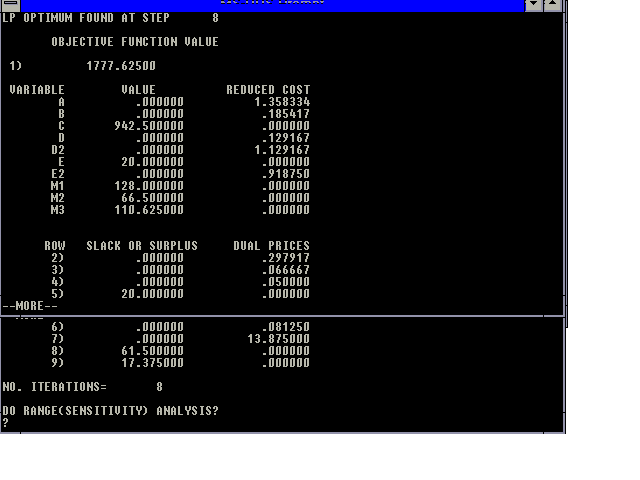
Note that the principal complication is that the profit contributions of products D and E are not linear. A technique to eliminate this problem is the definition of 2 products called D2 and E2 which sell for $3 per unit and constrain both D and E to less than or equal to 20 units per week.

First define the decision variables. The following table summarizes the decision variables.

Define                                  Profit Contribution/Unit

A: no. of units of A produced/week             5-2=$3
B: no. of units of B produced/week             4-1=$3
C: no. of units of C produced/week             5-2=$3
D: no. of units of D not in excess
   of 20 produced/week                         4-1=$3
D2: no. of units of D produced in
    excess of 20 per week.  Total
    production of product D is D + D2          3-1=$2
E: no. of units of E not in excess
   of 20 produced/week                         4-1=$3
E2: no. of units of E produced in
    excess of 20                               3-1=$2
M1: hours of machine 1 used per week              -$4
M2: hours of machine 2 used per week              -$4
M3: hours of machine 3 used per week              -$3

The objective function is:

profit=3A + 3B + 3C + 3D + 2D2 + 3E + 2E2 - 4M1 - 4M2 - 3M3

The constraints are:

12A + 7B + 8C + 10D + 10D2 + 7E + 7E2 - 60M1 = 0
8A + 9B + 4C + 11E + 11E2 - 60M2 = 0
5A + 10B + 7C + 3D + 3D2 + 2E + 2E2 - 60M3 = 0
D < = 20
E < = 20
M1 < = 128
M2 < = 128
M3 < = 128

The solution to this problem is shown in the graphic below.

Staff Covering Example Problem

     Hours              Collectors Needed
12 am - 6 am                    2
6 am to 10 am                   8
10 am to noon                   4
noon to 4 pm                    3
4 pm to 6 pm                    6
6 pm to 10 pm                   5
10 pm to mid night              3

Each collector works 4 hours, is off one hour (break), and then works another 4 hours. A collector can be started at any hour. Assuming the objective is to minimize the number of collectors hired, formulate the appropriate LP and find the number of workers to hire.

The decision variables are:

X1 = number of collectors to start work at 12 midnight
X2 = number of collectors to start work at 1 am
....
X24 = number of collectors to start work at 11 pm

The objective is to minimize the number of collectors hired. Therefore, the objective function is:

Minimize X1 + X2 + X3 + .... + X24

The constraint equations are:

X1 + X24 + X23 + X22 + X20 + X19 + X18 + X17 > = 2 
(For midnight to 1 am - note X21 not included since on break)

X2 + X1 + X24 + X23 + X21 + X20 + X19 + X18 > = 2 
(For 1 am to 2 am)

.....

X24 + X23 + X22 + X21 + X19 + X18 + X17 + X16 > = 3
(For 11 pm to midnight)

The results are:

Objective function value is 15.75

X1=0
X2=5
X3=0.75
X4=0.75
X5=0.75
X6=0.75
X7=0.75
X8=0
X9=0
X10=0
X11=1
X12=0
X13=0
X14=1
X15=2
X16=1
X17=1
X18=1
X19=0
X20=0
X21=0
X22=0
X23=0
X24=0

Note that the answer is not directly useful because some of the values are fractional. The value 15.75 implies that one should hire at least 16 collectors. This result is obtained by rounding the solution so an integer is obtained, for example by setting X3=X4=X6=X7=1 and X5=0.

Note that for problems of this type, that if the shifts contain no or very few breaks, then the LP solution will tend to be integer without resorting to integer programming.

Example Blending Problem

                     At Least    Not More Than
Carbon Content        3.0%            3.5%
Chrome Content        0.3%            0.45%
Manganese Content     1.35%           1.65%
Silicon Content       2.7%            3.0%

The steel company has the following materials available from which to produce this new steel:

                                                     Amount
        Cost/lb  Carbon  Chrome  Manganese  Silicon Available

Iron1     .03     4.0%     0%      0.9%      2.25%  unlimited
Iron2     .0645    0      10.0     4.5      15.0    unlimited
Fe-Sil1   .065     0       0        0       45.0    unlimited
Fe-Sil2   .061     0       0        0       42.0    unlimited
Alloy1    .10      0       0      60.0      18.0    unlimited
Alloy2    .13      0      20.0     9.0      30.0    unlimited
Alloy3    .119     0       8.0    33.0      25.0    unlimited
Carbide   .08    15.0      0        0       30.0      20 lb
Steel1    .021    0.4      0       0.9        0      200 lb
Steel2    .02     0.1      0       0.3        0      200 lb
Steel3    .0195   0.1      0       0.3        0      200 lb

The decision variables represent each of the materials available to produce the new steel. Let I1 represent Iron1, ..., and S3 represent Steel3.

The objective function is:

Minimize .03I1 + .0645I2 + .065F1 + .061F2 + .10A1 + .13A2 
         + .119A3 + .08C + .021S1 + .02S2 + .0195S3

The constraints come from the quality limits (upper and lower content limits), material availability, and the total weight of materials used must total 2000 lb. Thus the constraints are:

.04I1 + .15C + .004S1 + .001S2 + .001S3 < = (2000)(.035)
.10I2 + .20A2 + .08A3 < = (2000)(.0045)
.009I1 + .045I2 + .60A1 + .09A2 + .33A3 + .009S1 + .003S2 
  + .003S3 < = (2000)(.0165)
.0225I1 + .15I2 + .45F1 + .42F2 + .18A1 + .30A2 + .25A3
  + .30C < = (2000)(.03)
.04I1 + .15C + .004S1 + .001S2 + .001S3 > = (2000)(.03)
.10I2 + .20A2 + .08A3 > = (2000)(.003)
.009I1 + .045I2 + .60A1 + .09A2 + .33A3 + .009S1 + .003S2 
  + .003S3 > = (2000)(.0135)
.0225I1 + .15I2 + .45F1 + .42F2 + .18A1 + .30A2 + .25A3
  + .30C > = (2000)(.027)
C < = 20
S1 < = 200
S2 < = 200
S3 < = 200
I1 + I2 + F1 + F2 + A1 + A2 + A3 + C + S1 + S2 + S3 = 2000

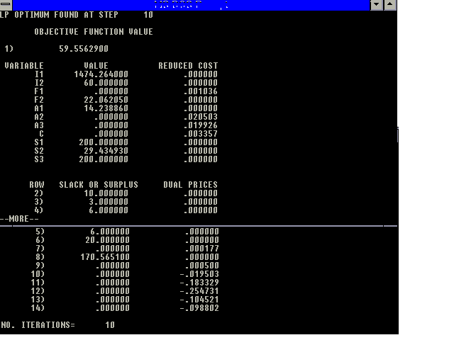
The solution is shown in the figure below.

Example Network Problem

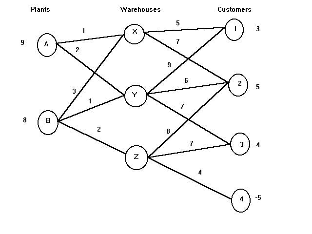
The firm has 2 plants (A and B), 3 warehouses (X, Y and Z) and 4 customer areas (1, 2, 3 and 4). The numbers adjacent to each node denote the availability of material at the node. For example, plant A has 9 units available to be shipped and customer 3 has -4 units (needs 4 units shipped in).

The number above each arc represents the cost per unit shipped along the arc. For example, if 5 of plant A's 9 units are shipped to warehouse Y, a cost of 5 x 2 = 10 is incurred. The problem is to determine the amount shipped along each arc so that total costs are minimized and every customer has their requirements filled.

The main condition of an LP for it to be a network problem is that it be representable as a network. There can be more than 3 levels of nodes and any number of arcs between any 2 nodes and limits may be placed on the amount shipped along an arc.

We will start the example problem by defining the decision variables. Let AX represent the units shipped along the link from plant A to warehouse X. Other variables are similarly defined and will be: AX, AY, BX, BY, BZ, X1, X2, Y1, Y2, Y3, Z2, Z3, and Z4.

The objective function is:

Minimize AX+2AY+3BX+BY+2BZ+5X1+7X2+9Y1+6Y2+7Y3+8Z2+7Z3+4Z4

A constraint is defined for each node such that sources=uses. Thus, the constraints are:

AX+AY=9
BX+BY+BZ=8
-AX-BX+X1+X2=0
-AY-BY+Y1+Y2+Y3=0
-BZ+Z2+Z3+Z4=0
-X1-Y1=-3
-X2-Y2-Z2=-5
-Y3-Z3=-4
-Z4=-5

The results are shown in the figure below.

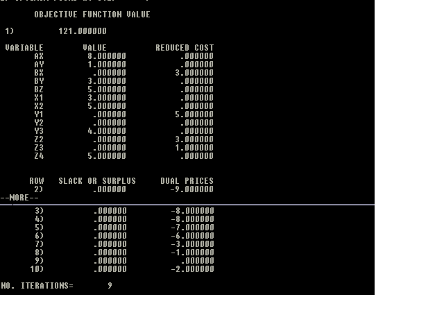
The solution exhibits 2 pleasing features which are found in the solutions of any network problem:

1. If the righthand side coefficients (the capacities and requirements) are integer, then so will be the variables.
2. If the objective coefficients are integer, then so will be the dual prices.

Network LPs can be summarized as follows:

1. Associated with each node is a number which specifies the amount of commodity available at that node (negative implies that commodity is required).
2. Associated with each arc are:
   • a cost per unit shipped (which may be negative) over the arc
   • a lower bound on the amount shipped over the arc (typically zero)
   • an upper bound on the amount shipped over the arc

The problem is to determine the flows which minimize total cost subject to satisfying all the supply, demand, and flow constraints.

Vertically Integrated Example Problem

The following table summarizes other features of the operation.

             Labor,
Activity  Machinery and     Water        Land        Alfalfa
           Other Costs   Requirements Requirements Requirements

wheat (ac)    $ 12         1.5 ac-ft      1 ac       
alfalfa (ac)    16         2.5 ac-ft      1 ac
1 ton beef     145         0.3 ac-ft     0.18 ac       5 tons

Vertically integrated problems such as this can be easily formulated if one carefully:

1. Identifies the activities whose levels are to be determined (i.e. identify the decision variables)
2. Identifies the commodities which are produced or consumed by the various activities. There will usually be one "sources=uses" or "material balance" constraint for each commodity.

If we observe that any wheat or beef which is raised will also be sold, then the activities/decision variables can be identified as:

wheat = wheat raised and sold (acres)
alfgrow = alfalfa raised (tons)
beef = beef raised and sold (tons)
alfbuy = alfalfa bought (tons)
alfsold = alfalfa sold (tons)

The commodities can be identified by describing the effect of each activity:

• Raising alfalfa uses dollars, land and water and produces alfalfa.
• Raising beef uses dollars, land, water and alfalfa and produces beef.
• Selling wheat, alfalfa, or beef uses wheat alfalfa, or beef and produces dollars.

Thus the commodities are land, water, and alfalfa with the commodity "dollars" being maximized. There will be constraints describing the usage of land, water and alfalfa.

The objective function is:

maximize 180.5wheat-3.2alfgro+755beef-78alfbuy+75alfsold

The constraints are:

wheat+.2alfgro+.18beef < = 1000   (land constraint)
1.5wheat+.5alfgro+.3beef < = 2200 (water)
-alfgro+5beef-alfbuy+alfsold = 0 (alfalfa)

The solution is shown in the figure below.

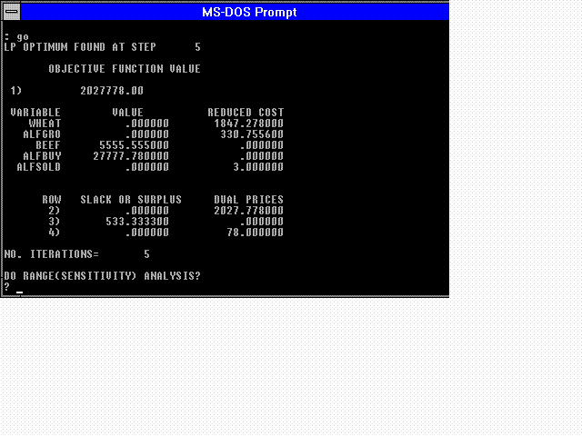
Note that the solution recommends that the entire farm be converted into a cattle feedlot. If this model is a preliminary one, then at this point one would raise questions about constraints which should be added. For example, it may be obvious that a labor constraint is needed. Most model development is iterative and constraints are added as there absence becomes obvious.