Assignment:

Read handout titled "Linear Programming."

Find a journal article in which linear programming was used to solve a problem. Read the article and prepare a brief (several paragraph) review. Email the review to the course instructor (engelb) by class time on Friday of week 3. (10 points)

Problems - Due End of Week 3

30 points

Problems are due Fri of week 3 by class time.

1. A rock quarry has two pits from which it obtains rock. The rock is run through a crusher to produce 2 products: concrete grade stone and road surface chat. Each ton of rock from the south pit converts to 0.75 tons of stone and 0.25 tons of chat when crushed. Rock from the north pit is of different quality and produces 50% of each type when crushed. The quarry has contracts for 60 tons of stone and 40 tons of chat this planning period (note this is the minimum amount that must be produced). The cost per ton of extracting and crushing the rock from the south pit is 1.6 times as costly as from the north pit.
   1. What are the decision variables for the problem?
   2. State the 2 constraints.
   3. Graph the feasible region.
   4. Draw an appropriate iso-cost (line of equal cost) on the graph and indicate graphically and numerically the optimal solution.
   5. Suppose all the information given in the problem description is accurate. What additional information might you nevertheless wish to know before having confidence in this model?
2. An equipment manufacturer produces two products, a field cultivator and a chisel plow, which share production facilities. Raw materials cost $600 per field cultivator and $750 per chisel plow. The field cultivator requires 4 hours in the foundry/forge area per unit and the chisel plow requires 2 hours per unit in the foundry/forge area. The field cultivator requires 2 hours in the assembly portion of the production facility and the chisel plow requires 3 hours in the assembly portion of the plant. The available daily capacities are 160 hours in the foundry/forge area and 180 hours in the assembly portion of the facility. The selling price of each field cultivator at the factory door is $4800 and that of the chisel plow is $5250. Whatever number of each type of equipment that can be produced at this factory can be sold.
   1. Write the objective function.
   2. Write the constraints.
   3. The above description assumes that the capacities of the forge/foundry and assembly line are sunk costs. Reformulate the LP under the conditions that each hour of foundry/forge time costs $95 while each hour of assembly line time costs $65. The capacities remain as before. Unused capacity has no charge.
3. A town is considering operating a materials recovery center (MRC) where paper can be separated and sold from municipal solid waste (MSW) for $25 per ton. The town generates 10,000 tons of MSW per year. Fifty percent of the solid waste is recyclable paper. The tipping fees are $10 per ton at the MRC and $50 per ton at the landfill. Note that materials not recycled at the MRC must be sent to the landfill. Assume all shipping fees are equal to zero. Given the above information, would you recommend operating the MRC? Show your work including a simple network diagram.

What is Linear Programming?

(For rigorous definitions and theory, which are beyond the scope of this document, the interested reader is referred to the many LP textbooks in print, a few of which are listed in the references section.)

A Linear Program (LP) is a problem that can be expressed as follows (the so-called Standard Form):

    minimize   cx
    subject to Ax  = b
                x >= 0

The word "Programming" is used here in the sense of "planning"; the necessary relationship to computer programming was incidental to the choice of name. Hence the phrase "LP program" to refer to a piece of software is not a redundancy, although I tend to use the term "code" instead of "program" to avoid the possible ambiguity.

Although all linear programs can be put into the Standard Form, in practice it may not be necessary to do so. For example, although the Standard Form requires all variables to be non-negative, most good LP software allows general bounds l <= x <= u, where l and u are vectors of known lower and upper bounds. Individual elements of these bounds vectors can even be infinity and/or minus-infinity. This allows a variable to be without an explicit upper or lower bound, although of course the constraints in the A-matrix will need to put implied limits on the variable or else the problem may have no finite solution. Similarly, good software allows b1 <= Ax <= b2 for arbitrary b1, b2; the user need not hide inequality constraints by the inclusion of explicit "slack" variables, nor write Ax >= b1 and Ax <= b2 as two separate constraints. Also, LP software can handle maximization problems just as easily as minimization (in effect, the vector c is just multiplied by -1).

The importance of linear programming derives in part from its many applications (see further below) and in part from the existence of good general-purpose techniques for finding optimal solutions. These techniques take as input only an LP in the above Standard Form, and determine a solution without reference to any information concerning the LP's origins or special structure. They are fast and reliable over a substantial range of problem sizes and applications.

Two families of solution techniques are in wide use today. Both visit a progressively improving series of trial solutions, until a solution is reached that satisfies the conditions for an optimum. Simplex methods, introduced about 50 years ago, visit "basic" solutions computed by fixing enough of the variables at their bounds to reduce the constraints Ax = b to a square system, which can be solved for unique values of the remaining variables. Basic solutions represent extreme boundary points of the feasible region defined by Ax = b, x >= 0, and the simplex method can be viewed as moving from one such point to another along the edges of the boundary. Barrier or interior-point methods, by contrast, visit points within the interior of the feasible region. These methods derive from techniques for nonlinear programming that were developed and popularized in the 1960s by Fiacco and McCormick, but their application to linear programming dates back only to Karmarkar's innovative analysis in 1984.

The related problem of integer programming (or integer linear programming, strictly speaking) requires some or all of the variables to take integer (whole number) values. Integer programs (IPs) often have the advantage of being more realistic than LPs, but the disadvantage of being much harder to solve. The most widely used general-purpose techniques for solving IPs use the solutions to a series of LPs to manage the search for integer solutions and to prove optimality. Thus most IP software is built upon LP software, and this FAQ applies to problems of both kinds.

Linear and integer programming have proved valuable for modeling many and diverse types of problems in planning, routing, scheduling, assignment, and design. Industries that make use of LP and its extensions include transportation, energy, telecommunications, and manufacturing of many kinds. A sampling of applications can be found in many LP textbooks, in books on LP software systems, and among the application cases in the journal Interfaces.

Important Terms and Concepts:

Objective function - function defined within an LP problem that is to be maximized or minimized; often called the profit function.

constraints - limitations placed on the decision variables in an LP problem

decision variables - variables that comprise the objective function of a LP

slack variable - used to convert LP constraint equality of type 1 (<=) to an equation; a non-negative variable (slack variable) is added to such an inequality to produce an equation; For example, 3X1 + X2 - 2X3 <= 10 becomes 3X1 + X2 - 2X3 + X4 = 10 when X4 is added as a slack variable.

surplus variable - used to convert LP constraint inequality of type 2 (>=) to an equation; For example 4X1 + 2X2 >= 10 becomes 4X1 + 2X2 - X3 = 10 when a non-negative surplus variable is subtracted from the left hand side.

Note that most LP solvers convert inequalities to equations using slack and surplus variables prior to solving the objective function.

Simplex Method - the most widely used procedure for solving LP problems; commonly used within computer-based LP solvers

Linear Programming (LP) is a mathematical procedure for determining optimal allocation of scarce resources. LP has found practical application in nearly all facets of business. Transportation, distribution, and aggregate production planning problems are the most typical objects of LP analysis. Within agriculture, LP has been widely used for allocation of limited resources (selection of crop land mix), allocation of limited resources with time (irrigation), formulation of least cost rations (animal feed), and transportation.

It is important to note that "programming" in LP is quite different than programming in a computer language such as C or FORTRAN. With LP, the bulk of the effort is in formulating the problem.

In LP problems, there are two types of objects: "limited resources" such as land, labor, capital, or plant capacity; and "activities" such as "produce corn flakes" or "produce widgets". Each activity consumes or possibly contributes additional amounts of the resources. The problem is to determine the best combination of activity levels which does not use more resources than are actually available.

The following approach is normally followed in formulating a model to be solved with linear programming:

1. Define the control or decision variables
2. Establish the objective function
3. Establish constraints placed on the system

The constraint set of an optimization model model serve two major purposes:

1. It simulates the system or process under investigation.
2. It is a statement of restrictions reflecting policy, resources, budgetary, and other limiting factors.

The following example will demonstrate a simple LP example to provide a better understanding of how such problems might be formulated and solved.

A Simple Product Mix LP Example

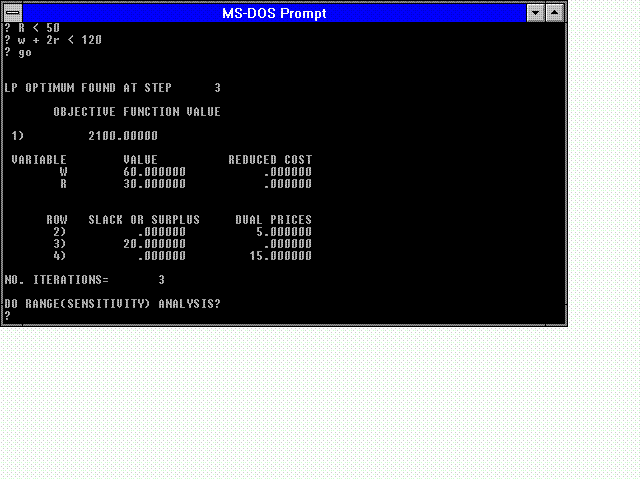
First, let W represent the number of wind speed sensors and R represent the number of rainfall sensors. The second step is to define and write the objective function. The objective function is:

Maximize 20W + 30R

Next the resource constraints are defined. In this case, there are two types of constraints: on labor and on the production capacity of the production lines.

W < = 60        (wind speed sensor line capacity)
R < = 50        (rainfall sensor line capacity)
W + 2R < = 120  (labor)

In addition to the above constraints, most LP solver computer programs assume the constraint variables are nonnegative (i.e., W >= 0 and R >= 0).

The constraints for the above problem are plotted in the diagram below.

For the problem above, the objective function is maximized when 60 wind speed sensors and 30 rainfall sensors are produced.

Linearity

1. The effects of a single variable or activity by itself are proportional; e.g., doubling the amount of steel produced will double the dollar amount of steel sold, the amount of electricity to produce the steel, etc., regardless of the current level of steel produced
2. The interactions among variables must be additive; e.g., the dollar amount of sales is the sum of the steel dollar sales, the aluminum dollar sales, etc., while the amount of electricity used is the sum of that used to produce steel, aluminum, etc.
3. The variables must be continuous; i.e., fractional values for the decision variables, such as 3.46, must be allowed.

Outcomes (Solutions) to LP Problems

1. Single unique optimum solution
2. Multiple optimum solutions
3. No feasible solution
4. Unbounded solution

Sensitivity Analysis

Many LP solvers provide information concerning the sensitivity of the solution if requested. The figure below shows the solution for our example problem above.

The figure that follows provides information concerning the sensitivity of the solution. For this particular example, the coefficient to the number of wind speed gages produced (the profit per wind speed gage) could decrease by 5 or increase to infinity without the solution changing while the coefficient (profit) for the rain gages could increase by 10 or decrease by 30 without the solution changing. The information for rows 2, 3, and 4 represent the constraints:

W < = 60        (wind speed sensor line capacity)
R < = 50        (rainfall sensor line capacity)
W + 2R < = 120  (labor)

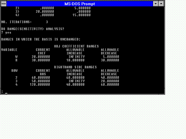
Using this information, one can determine how sensitive the solution obtained is - very often there are additional factors that can not easily be put in mathematical form that may influence a decision and thus the sensitivity analysis can be extremely valuable. The sensitivity analysis also provides information that is useful in understanding how well coefficients and constraints must be defined.