Week 11 - Neural Networks

Introduction to Neural Networks

Introduction

Neural networks have grown out of work in the field of artificial intelligence. Neural networks are an attempt to create an "artificial brain" and mimic the functionality of the human brain. Thus neural network terminology has many similarities with the anatomy of the human brain.

Neural network applications differ greatly from other computer-based approaches to problem solving in that an application is not programmed but rather the neural network is "taught" - this explains much of the popularity of neural networks.

What is a Neural Network?

In contrast, a neural network is neither sequential nor even necessarily deterministic. It has no separate memory array for storing data. The processors that make up a neural network are not highly complex central processing units. Instead, a neural network is composed of many simple processing elements that typically do little more than take a weighted sum of all its inputs. The neural network does not execute a series of instructions; it responds to the inputs presented to it. The result is not stored in a specific memory location, but consists of the overall state of the network after it has reached some equilibrium condition.

Knowledge within a neural network is not stored in a particular location. You can't look at memory address 1345 to retrieve the current value of the variable X. Knowledge is stored both in the way the processing elements are connected (the way the output signal of a processing element is connected to the input signals of many other processing elements) and in the importance (or weighting value) of each input to the processing elements. Knowledge is more a function of the network's architecture than the contents of a particular location.

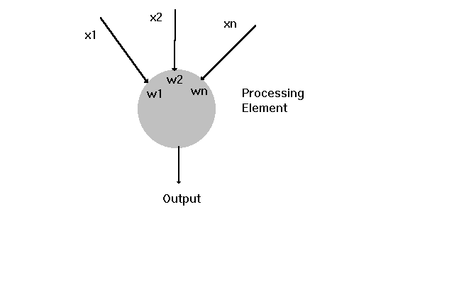
Two primary elements make up a neural network: processing elements and interconnections. Processing elements, the neural network equivalent of neurons, are generally simple devices that receive a number of input signals and, based on those inputs, either generate a single output signal (fire) or do not. The output signal of an individual processing element is sent to many other processing elements (and possibly back to itself) as input signals via the interconnections between processing elements.

The structure of the neural network is defined by the interconnection architecture between the processing elements, the rules that determine whether or not a processing element will fire (the transfer function), and the rules governing changes in the relative importance of individual interconnections to a processing element's input (training laws). Software that defines these aspects of a neural network's structure to generate a network and solve a specific problem is called netware or neural network simulation software.

A neural network software programmer does not specify an algorithm to be executed by each processing element, as a programmer of a more traditional computer program. Instead, the programmer specifies interconnections, transfer functions, and training laws of the network, then applies appropriate inputs to the network and lets it react. If the neural network software is correctly written, the overall state of the network after it has reacted to the input will be the desired response pattern.

This is quite different from standard programming. That is because neural networks are a completely different way of looking at computer systems. The biological inspiration shows up clearly in the terminology use for neural networks, as well as in the way we think about them. Neural networks don't "execute programs" as much as they "behave" given a specific input. They "react", "self organize", "learn" and "forget".

Why the Interest in Neural Networks?

It turns out that neural networks are good at solving the kinds of problems people can easily solve. They are also fairly terrible at solving the kinds of problems traditional computers do well but people solve slowly and inefficiently, if at all.

In general, neural networks do not do well at precise, numerical computations. On the other hand, this form of computation is not a natural application for people, either. Neural networks can however, be taught to determine whether or not a visual image of a face is that of a man or woman, or recognize a particular person's face, even with a different facial expression or hairdo People do this from the time they are babies, but this is difficult with more traditional computer programming techniques. The role of neural networks is best as partners to traditional systems, not a replacement for them.

Basics of Neurocomputing

The simplest kind of processing element compares this weighted sum input to an arbitrary threshold (T). This threshold value is often 0. If the input is greater than the threshold value, the processing element fires or generates an output signal. If the input is less than the threshold value, the processing element does not fire and no output is generated.

The next figure shows the output signal from the processing element is fanned out to act as inputs to a number of other processing elements. It can also act as one of the input signals to itself, depending on whether the network architecture requires direct feedback.

These outputs (and the corresponding input signals) can be either excitatory or inhibitory. An excitatory input means the signal tends to cause the processing element to fire; an inhibitory input means the signal tends to keep the processing elements from firing. Excitatory inputs are often positively weighted and valued, while inhibitory inputs are negatively weighted and valued.

The inputs and the weights can be viewed as vectors with components of (x1, x2, ..., xn) and (w1, w2, ..., wn), respectively. If we do this, the total input signal is just the dot product of the weight vector and the input vector.

From analytical geometry, we know that the dot product of two vectors is also equivalent to the projection of one vector onto the other vector. Mathematically, the dot product is equivalent to |w| |x| cos B where |w| is the magnitude (size) of the vector w; |x| is the magnitude of vector x, and B is the angle between the two vectors.

This is very important because it gives us a visual image of what these vectors mean. The projection of the weight vector on the input vector will be greatest when the two vectors are pointed in almost the same direction, and smallest when the two vectors are pointed in very different directions. Essentially this is a measure of the closeness of the two vectors to each other. Thus, the input will be largest when the weight vector and the input vector are very close to each other. Suppose we had 5 different processing elements, each with the same set of input signals but different sets of weights on the input signals. Suppose we were only going to let one processing element fire - the one with the largest input signal. The processing element that fires is the one with a weight vector closest to the input vector. We can imagine the five processing elements with their weight vectors distributed in space, pointing in five completely different directions. The processing element that fires will be the one with the weight vector most nearly in the direction the input vector points. Keeping this visual image of weight vectors and input vectors in mind is extremely helpful in gaining insight into neural network's operation.

We have a primitive but useful system in the above example. Suppose we want a system that recognizes inputs and classifies them into one of five distinct patterns. All we have to do is set up the five processing elements with weight vectors that point to the classical versions of each of the five patterns we want to recognize. Then we present the input signal from some unknown sample to the inputs of each of the five patterns simultaneously. The processing element with the best match will fire with the greatest strength, and that tells us which pattern the input most closely remembers.

For example, we could have the processing elements output their net weighted input signals as a voltage, which we could wire into a light bulb. The bulb that burns brightest tells us which kind of pattern the input belonged to. Notice that this classification technique takes place in constant time, no matter how many possible classifications we have. All we need is one processing element per bin.

Learning in Neural Networks

The output is computed as a result of a transfer function of the weighted input. The net input for this simple case is computed by multiplying the value of each individual input by its corresponding weight, or equivalently, taking the dot product of the input and weight vectors. The processing element then takes this input value and applies the transfer function to it to compute the resulting output.

Normally the transfer function for a given processing element is fixed at the time a network is constructed. If we want to change the output value, we have to do something to change not the transfer function but the weighted input.

Since the processing element has no control over what input patterns are presented to it, it reacts to rather than creates its environment. The only means it has to change the weighted input is to modify the values of the weights on the individual inputs. Thus networks learn by changing the weights on the inputs. The learning law for a given network defines precisely how to change the weights in response to a given input and output pair.

Learning in neural networks can be supervised or unsupervised. Supervised learning means the network has some omniscient input present during training to tell it what the correct answer should be. The network then has a means to determine whether or not its output was correct and knows how to apply its particular learning law to adjust its weights. Unsupervised learning means the network has no such knowledge of the correct answer and thus cannot know exactly what the correct response should be.

Although both kinds of learning are important for different applications, only supervised learning is explored here.

One particular learning law is one of the most commonly used learning algorithm in neural nets. It is called the Delta rule or Least Mean Square (LMS) training law.

Neural Net Examples

Additional internet resources on neural networks: neural nets

activation function - A function by which new output of the basic unit is derived from a combination of the net inputs and the current state of the unit (the total input).

auto-associative (memory system) - A process in which the system has stored a set of information repeatedly presented to it. Later, when you submit a similar pattern to the system, it can recall the information from a degraded or incomplete version of the original.

axon - The part of a nerve cell through which impulses travel away from the cell body; the electrically active parts of a nerve-cell.

back-propagation - A learning algorithm for a multilayer network in which the weights are modified via the propagation of an error signal "backward" from the outputs to the inputs.

chaos - The study of nonlinear dynamics (also called deterministic disorder).

connection - A pathway between processing elements, either positive or negative, that links the processing elements into a network.

dendrite - The branched part of a nerve cell that caries impulses toward the cell body. The electrically passive parts of a nerve cell.

directed graph - Representation of the variation and direction of flow for processing elements with respect to other processing elements.

feedback loop - A loop wherein continued input is fed back into the network to achieve the expected output.

fuzzy logic - Incomplete or contradictory information.

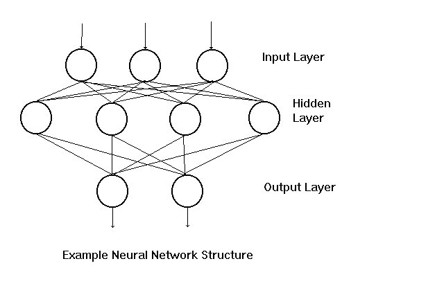
hidden layer - A third layer of units between the input and the output layers that provides additional computational power.

learning - The phase in a neural network when new data is introduced into the network, causing the weights on the processing elements to be adjusted.

network paradigm - A network architecture that specifies the interconnection structure of a network.

neuron - The structural and functional unit of the nervous system, consisting of the nerve cell body and all its processes, including an axon and one or more dendrons.

perceptron - A large class of simple neuron-like networks with only an input layer and an output layer. Developed in 1957 by Frank Rosenblatt, this class of neural network had no hidden layer.

sigmoid - Having a double curve like the letter S.

spreading activation - A process of applying the activation function simultaneously to a neural network.

stochastic - Involving chance, probability or a random variable.

summation function - A function that combines the various input activations into a single activation.

synapse - The point of contact between adjacent neurons where nerve impulses are transmitted from one to another.

threshold - A minimum level of excitation energy.

training - A process whereby a network learns to associate an input pattern with the correct answer.

weight - The strength of an input connection expressed by a real number. Processing elements receive input via interconnects. Each interconnect has a weight attached to it. The sum of the weights make up a value that updates the processing element. The output value of a processing element is described by a level of excitation that causes interconnects to be either on (i.e. excitatory output) or off (i.e. inhibitory output).