"Color calibration" for color classification
Definition of the problem
Color classification is sometimes very sensitive to illumination changes, and to setup changes in general (camera, lenses...). The perturbation shifts the color classes in the color space, thus making the carefully designed classifier (discriminant functions) useless. Different solutions exist to reduce the influence of such changes:- Reset the system to the training conditions
- Resampling the color classes and rebuilding the classifier
- Running a calibration to compensate for the changes
Solution 2. is the easiest. However, collecting the range of color variation for the problem can be long (many color variations in the problem), or impossible if the setup is sorting produces in real-time and cannot be stopped for retraining.
Solution 3. is the most elegant, using information on the new state of the system to transform the previoulsy developed color classifier.
Color shift example
This example was developed for a white seed corn sorting system we developed in the Agricultural Engineering Department for Pioneer Hi-Bred International. In the white seed corn sorting application the color classes are very close to one another to the point that only an expert white seed corn breeder can tell them apart...
Two system setups were designed using changes in illumination and aperture.
Five seeds are used to sample the 5 color classes:
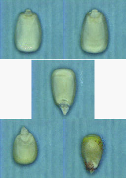
Figure 1: Setup 1-Five sorted white seed
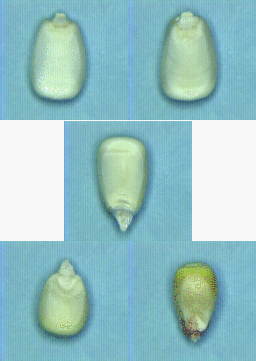
Figure 2: Setup 2-Five sorted white seed
The following 3D plot shows 7 different color classes in the RGB space
(0-background, 8-hard starch, 4 white classes (1-4) and 1 yellow class (5)),
sampled from the setup 2 image (using my Samplex software).
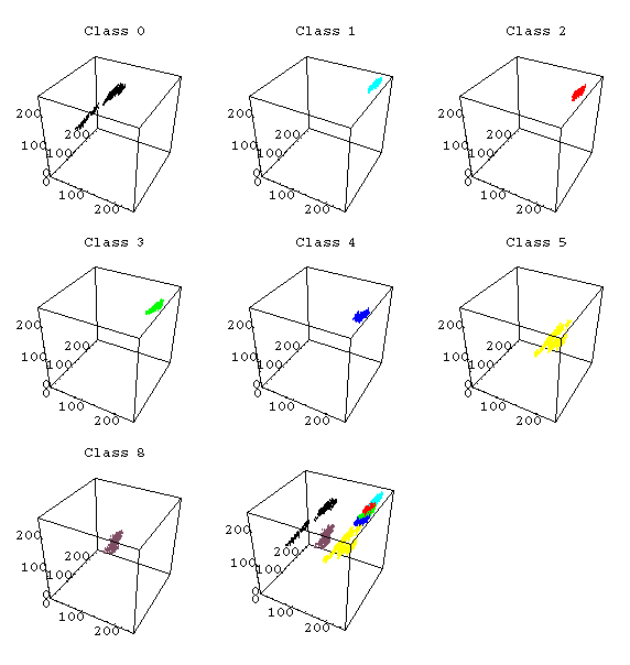
Figure 3: Color classes distribution in the RGB space.
For simplicity's sake the calibration procedure will be explained with just
2D data, the red and blue band.
An illustration of the shift in color is the plot of the normal distribution
for a certain percentage of the distribution. These plots were created with
a Mathematica package I wrote for displaying color class information.
The following graphs show the distribution in Red-Blue space. (Warning:
the ellipse's colors are not consistent with Figure 3).
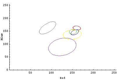
Figure 4: Theoretical normal distribution for 60% of the points setup 1
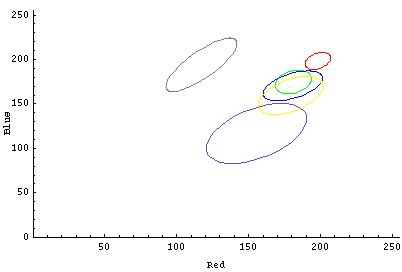
Figure 5: Theoretical normal distribution for 60% of the points setup 2
Plotting the two sets of normal distribution one can see the overlap from
one setup to the other. This render the classifier developed for setup 1
useless in the setup 2 conditions...
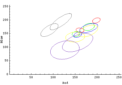
Figure 6: Distribution from setup 1 and 2
The classifier build for setup 1 is made of 5 linear discriminant functions
using the BLC2 neural network classifier of samplex.
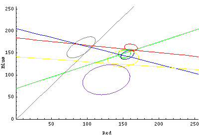
Figure 7: Distributions and discriminant planes for setup 1
The result of the color classification is the following:

Figure 8: Classification of setup 1 image with its classifier
Each kernel class has a different breakdown in color class. This classification system was tested on a large sample of white seed corn and compared with an expert classification. The vision system was 95% accurate.
Classifying the image of setup 2 with the setup 1 classifier leads to a poor
classification:
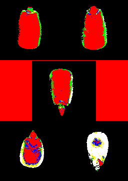
Figure 9: Classification of setup 2 image with setup 1 classifier
This classification is somewhat accurate for background and the yellow kernel class. However, no discrimination is achieved for the white seed corn classes.
Plotting the setup 1 classifier with the distributions from setup 2 illustrate
why the classification fails:
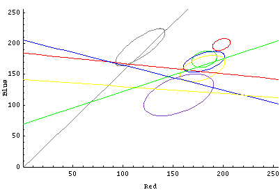
Figure 10: Distributions for setup 2 and discriminant planes for setup 1
Classifier transformation
In this color classification problem the objective is to transform a set of discriminant functions from one setup to another.The new distribution information can be acquired using a "color standard" made of white corn kernels or manufactured color plates. When using a white corn standard the data obtained is new distributions for each color class.
The transformation operation is a matrix B computed from the covariance
matrices and mean vectors from each setup. A point P transformation from
one setup to the next is P'= P.B
The transformation matrix is computed
using a multivariate multilinear regression.
The following figure presents the discriminant planes of setup 1 transformed to fit the new distribution of setup 2:
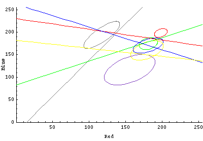
Figure 11: Transformed discriminant planes and setup 2 distributions
Calibration results analysis
The calibration results can be analyzed by comparing the resubstitution error of the discriminant planes on the setup 1 distributions and the transformed planes on the setup 2.
        Total error 18.46%
        Confusion Matrix
        0       1       2       3       4       5
0       1220    0       0       0       0       0
1       0       219     40      16      0       0
2       0       22      207     186     159     0
3       0       25      47      591     287     0
4       0       0       58      132     724     20
5       0       0       0       0       23      1521
Table 1: Confusion matrix for setup 1 data
        Total error 19.60%
        Confusion Matrix
        0       1       2       3       4       5
0       4448    0       0       0       0       0
1       0       550     1       0       0       0
2       0       58      198     416     326     0
3       0       34      42      466     601     2
4       0       0       5       223     881     220
5       0       0       0       0       29      1484
Table 2: Confusion matrix for setup 2 data with discriminant planes transformed
from setup 1The difference in resubstitution error is 1.2%.
The classification of the setup 2 image can also be used for a visual estimation. The results of this classification yielded correct classification for each kernel.
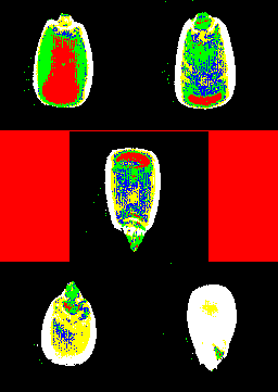
Figure 12: Setup 2 image classified with transformed classifier