Numerical integration (A)
Goals
The goals of this assignment are as follows:
- How to calculate the Fourier coefficients of a Fourier series associated with a function
- How to define a structure needed
- How to use argc and argv correctly in main.
Getting Started
Start by getting the files. Type 264get hw05 and then
cd hw05 from bash.
You will get the following files:
- fourier.c: this is the file that you hand in. It has the description of the numerical integration method in HW04, the description of an extension of it for computing the integrand needed for Fourier coefficients, and the description of a function to compute Fourier coefficients. You must hand in this file.
- fourier.h: this is a "header" file and it declares the functions that you will be writing for this assignment. You also have to define the structure required. You must hand in this file.
- main.c: You should use this file to write the main function that would properly initialize the structure that would be passed into the function to compute Fourier coefficients.
- aux.h: an include file to declare a few unknown functions for which you have to calculate their associated Fourier coefficients.
- aux.o: provide the object code for the unknown functions declared in aux.h.
- util.h: an include file to declare utility functions for you to use in printing and also to plot functions in matlab format.
- util.c: definition of functions declared in util.h.
- plots: This folder contains 6 files which are plots for
unknown_function_3: data5.m, data10.m, data20.m, data40.m, data80.m, and data160.m. These plots are in matlab format.
To get started, read this homework description in its entirety. Browse through the fourier.h and fourier.c files to see what code needs to be written. You will be writing code in the fourier.c file. You will also write code in the main.c file to call the functions in fourier.c. Both fourier.c and main.c contain comments that tell you the code that needs to be written in fourier.c and main.c, respectively. You should also read both fourier.c and main.c to figure out the structure that needs to be defined in fourier.h.
Follow the discussions below on how to compile and run your code, as well as test and submit it.
Submitting Your Assignment
You must submit three files:
- fourier.h
- fourier.c
- main.c
Submit
To submit HW05, type
264submit HW05 fourier.h fourier.c main.c
from inside your hw05 directory.
Fourier Series
In the CompE and EE curricula in ECE, all students have to take the course ECE 301 Signals and Systems. In ECE 301, a Fourier Series is typically expressed in the form of complex exponential. In this assignment, we will deal with the form that has terms that are more familiar to you: sine and cosine. While ECE 301 will teach you the mathematics that ground the Fourier series, which requires many derivations, this assignment shows you how to perform the numerical calculation to obtain a Fourier series.
The following is based on the materials taken from here (Professor Peter J. Olver, Head of the School of Mathematics, University of Minnesota) and here (late Dr. James Stewart, most recently Professor of Mathematics at McMaster University). You can also find the resource of Fourier series on Wolfram and wiki.
Why do we have to know Fourier Series. The following two paragraphs are lifted from Professor Peter Olver's write up:
"Just before 1800, the French mathematician/physicist/engineer Jean Baptiste Joseph Fourier made an astonishing discovery. As a result of his investigations into the partial differential equations modeling vibration and heat propagation in bodies, Fourier was led to claim that “every” function could be represented by an infinite series of elementary trigonometric functions — sines and cosines. As an example, consider the sound produced by a musical instrument, e.g., piano, violin, trumpet, oboe, or drum. Decomposing the signal into its trigonometric constituents reveals the fundamental frequencies (tones, overtones, etc.) that are combined to produce its distinctive timbre. The Fourier decomposition lies at the heart of modern electronic music; a synthesizer combines pure sine and cosine tones to reproduce the diverse sounds of instruments, both natural and artificial, according to Fourier’s general prescription."
"Fourier analysis is an essential component of much of modern applied (and pure) mathematics. It forms an exceptionally powerful analytical tool for solving a broad range of partial differential equations. Applications in pure mathematics, physics and engineering are almost too numerous to catalogue — typing in “Fourier” in the subject index of a modern science library will dramatically demonstrate just how ubiquitous these methods are. Fourier analysis lies at the heart of signal processing, including audio, speech, images, videos, seismic data, radio transmissions, and so on. Many modern technological advances, including television, music CD’s and DVD’s, video movies, computer graphics, image processing, and fingerprint analysis and storage, are, in one way or another, founded upon the many ramifications of Fourier’s discovery. In your career as a mathematician, scientist or engineer, you will find that Fourier theory, like calculus and linear algebra, is one of the most basic and essential tools in your mathematical arsenal. Mastery of the subject is unavoidable."
In reality, every piecewise continuous function $f$ over a range $[a, b]$ can have a Fourier series $F$ associated with it. However, that does not mean that $f$ is equal to $F$. However, if $f$ is a periodic with period (b - a) and $f$ and its derivative are continuous over $[a, b]$, $f$ is equal to $F$ where $f$ is continuous. Where $f$ is discontinuous at $x$, $F(x)$ is the average of the right and left limits, i.e., $F(x) = \frac{f(x^+) + f(x^-)}{2}$ (the values of the function $f$ as we get closer and closer to x from its right and left).
A function $f$ is said to be periodic if the function $f(x)$ repeats itself in regular intervals or periods. A sine wave or cosine wave is periodic, with the period being $2 * \pi$, where $\pi$ is the mathematical constant that defines the ratio of a circle's circumference to its diameter. (In C, the macro M_PI defines the numeric value of $\pi$ in math.h.)
Typically, the Fourier series is expressed over a range $[-\pi, \pi]$. We provide the general representation here, where f is defined over a range $[a, b]$. If $f$ is assumed to be periodic on interval $[a, b]$, with $2L = (b - a)$ being the period,
$ F(x) = \frac{a_0}{2} + \sum_{n = 1}^{ \infty} a_n \cos(\frac{n * \pi * x}{L}) + \sum_{n = 1}^{\infty} b_n \sin(\frac{n * \pi * x}{L}) $ ,where $\sum_{n = 1}^{ \infty}$ is the summation of terms with n = 1, 2, ... till infinity, $\cos$ is the cosine function, and $\sin$ is the sine function.Therefore, $\sum_{n = 1}^{ \infty} a_n \cos(\frac{n * \pi * x}{L}) = a_1 \cos(\frac{1 * \pi * x}{L}) + a_2 \cos(\frac{2 * \pi * x}{L}) + ...$ In the Fouries, $a_0, a_1, a_2$, ..., and $b_1, b_2$, ... are the Fourier coefficients, which are defined as follows:
$a_0 = \frac{1}{L} * \int_{a}^{b} f(x) dx$where $\int_{a}^{b}$ is the integration over the interval $[a, b]$. Your task in this assignment is to write a C function and its related functions to compute $a_0, a_1, a_2, ...$ and $b_1, b_2, ...$
$a_n = \frac{1}{L} * \int_{a}^{b} f(x) \cos(\frac{n * \pi * x}{L}) dx, n = 1, 2, ...$
$b_n = \frac{1}{L} * \int_{a}^{b} f(x) \sin(\frac{n * \pi * x}{L}) dx, n = 1, 2, ...$
As a side note, when [$a, b] = [-\pi, \pi],$ we obtain the more familiar form of Fourier series (where $2L = 2\pi$, i.e., $L = \pi$): $F(x) = \frac{a_0}{2} + \sum_{n = 1}^{\infty} a_n \cos(n * x) + \sum_{n = 1 }^{\infty} b_n \sin(n * x) $ ,where $a_0 = (1/\pi) * \int_{-\pi}^{ \pi} f(x) dx$
$a_n = (1/\pi) * \int_{-\pi}^{ \pi} f(x) \cos(n * x) dx $
$b_n = (1/\pi) * \int_{-\pi}^{ \pi} f(x) \sin(n * x) dx $
Why do we care about periodic functions? Many astronomical phenomena are periodic in nature. The rotation of the moon around Earth, our heartbeats, and vibrating strings are some examples. Even for man-made objects, we can find periodic behavior. We rely on a periodic clock signal to synchronize the operations of registers or flip-flops in an integrated circuit.
If we are to design a synthesizer that can play different types of musical instruments, we have to obtain the Fourier series of a particular instrument when a particular note is played so that we can use the Fourier series to re-construct the sound made by that instrument. All we have to do is make sure that we can generate sine and cosine waves and we can then combine (add) these waves (weighted by appropriated $a_1, a_2, ...$, and $b_1, b_2, ...$).
Of course, it is impossible to combine an infinite series. Therefore, we typically approximated the Fourier series with only the first (k+1) terms (if we start the index at $a_0$ and end the index at $a_k$):
$ F(x) ~ a_0/2 + \sum_{n = 1}^{k} a_n \cos(\frac{n * \pi * x}{L}) + \sum_{n = 1}^{k} b_n \sin(\frac{n * \pi * x}{L}) $ , whereThe computation of $a_0, a_n,$ and $b_n$ involves integration, a topic that you have dealt with in HW03 and HW04. In particular, we will use the Simpson's method in HW04 in this assignment.
$a_0 = \frac{1}{L} * \int_{a}^{b} f(x) dx$
$a_n = \frac{1}{L} * \int_{a}^{b} f(x) \cos(\frac{n * \pi * x}{L}) dx, n = 1, 2, ..., k $
$b_n = \frac{1}{L} * \int_{a}^{b} f(x) \sin(\frac{n * \pi * x}{L})dx, n = 1, 2, ..., k $
Functions and structure you have to define
Structure you have to define
In HW04, you have to been asked to define a structure called Integrand. You have to do the same here. Please read up on HW04 on that. As in HW04, this is the only change you can make to fourier.h. You are not allowed to make other changes in fourier.h. This structure will be used in another structure defined in fourier.h called fourier.
typedef struct _Fourier {
   Integrand intg;
   int n_terms;
   double * a_i;
   double * b_i;
} Fourier;
In the structure Fourier, we have Integrand, which is defined by you. The field n_terms stores the number of terms in the truncated Fourier series. If the coefficient with the highest index is k, the field n_terms should have a value of k+1.
The field $a_i$ stores an address pointing to a block of n_terms double's, and $a_i[0]$ corresponds to $a_0$, $a_i[1]$ corresponds to $a_1$, ..., and $a_i$[n_terms-1] corresponds to $a_{n\_terms-1}$. Therefore, if n_terms has a value of k+1, $a_i[k]$ corresponds to the coefficient with the highest index.
The field $b_i$ stores an address pointing to a block of n_terms double's, We do not use the first entry $b_i[0]$. Here, $b_i[1]$ corresponds $b_1, b_i[2]$ corresponds to $b_2, ...$, and $b_{i}[{n\_terms}-1]$ corresponds to $b_{n\_terms-1}$.
main.c contains code fragment that shows you how to allocate the space for $a_i$ and $b_i$. It also contains code fragment to free the space. Do not modify them. Modification to this code fragment may lead to memory errors.
2b. Functions you have to write in fourier.c
You have to write the following three functions. These three functions are declared in fourier.h:
double simpson_numerical_integration(Integrand intg_arg);

double simpson_numerical_integration_for_fourier(Integrand intg_arg, int n, double (*cos_sin)(double));

void fourier_coefficients(Fourier fourier_arg);
If you have to write additional function, please declare and define your functions in fourier.c. DO NOT declare your functions in fourier.h. There are two locations in fourier.c where you want to declare and define your functions.
You may declare and define functions between these two lines found in fourier.c.
// IF YOU HAVE TO declare and define more functions, do so between this line
// and this line
You may also define functions at the end of the file fourier.c after the following line:
// IF YOU HAVE TO define more functions, do so after this line
Simpson's rule integration method
The function simpson_numerical_integration(Integrand intg_arg) computes
$\int_{a}^{b} f(x) dx$
Note that all information necessary for the integration should be contained
in intg_arg. This should be the same as that in HW04. Simply copy that over.
For the following integrations:
$\int_{a}^{b} f(x) \cos(\frac{n * \pi * x}{L}) dx, n = 1, 2, ..., k $The function
$\int_{a}^{b} f(x) \sin(\frac{n * \pi * x}{L}) dx, n = 1, 2, ..., k $
where 2L = (b - a)
 simpson_numerical_integration_for_fourier(Integrand intg_arg,
int n, double (*cos_sin)(double))
should be used. Note that the function
being integrated is
$f(x) \cos(\frac{n * \pi * x}{L}) $
or
$f(x) \sin(\frac{n * \pi * x}{L}) $
The function $f(x)$ is contained in intg_arg. The parameter n (int) supplied
to simpson_numerical_integration_for_fourier(…) corresponds to the n in the
$\cos$ or $\sin$ function. $\pi$ is define in math.h as M_PI. The address
cos_sin supplied to the funciton simpson_numerical_integration_for_fourier(…)
is either the address of the function sin or the address of the function
cos, both of which are declared in math.h and available in the math library.
The caller will decide which function, sin(…) or cos(…), to send to the function.
Both simpson_numerical_integration(…) and
simpson_numerical_integration_for_fourier(…) are similar in the flow.
The only difference is one is computing $f(x)$ and the other one is
computing
$f(x) \cos(\frac{n * \pi * x}{L}) $
or
$f(x) \sin(\frac{n * \pi * x}{L}) $
2b-ii. Computing Fourier coefficients
The function simpson_numerical_integration(Integrand intg_arg) computes
$\int_{a}^{b} f(x) dx$
Note that all information necessary for the integration should be contained
in intg_arg. This should be the same as that in HW04. Simply copy that over.
For the following integrations:
$\int_{a}^{b} f(x) \cos(\frac{n * \pi * x}{L}) dx, n = 1, 2, ..., k $ $\int_{a}^{ b} f(x) \sin(\frac{n * \pi * x}{L}) dx, n = 1, 2, ..., k $ where $2L = (b - a)$,The function
simpson_numerical_integration_for_fourier(Integrand intg_arg,
int n, double (*cos_sin)(double)) should be used. Note that the function
being integrated is
$f(x) \cos(\frac{n * \pi * x}{L}) $
or
$f(x) \sin(\frac{n * \pi * x}{L}) $
The function $f(x)$ is contained in intg_arg. The parameter n (int) supplied
to simpson_numerical_integration_for_fourier(…) corresponds to the n in the
$\cos$ or $\sin$ function. $\pi$ is define in math.h as M_PI. The address
cos_sin supplied to the funciton simpson_numerical_integration_for_fourier(…)
is either the address of the function sin(…) or the address of the function
cos(…), both of which are declared in math.h and available in the math library.
The caller will decide which function, sin or cos, to send to the function.
Both simpson_numerical_integration(…) and
simpson_numerical_integration_for_fourier(…) are similar in the flow.
The only difference is one is computing $f(x)$ and the other one is
computing $f(x) \cos(\frac{n * \pi * x}{L}) $
or
$f(x) \sin(\frac{n * \pi * x}{L}) $
The main function
The executable of this exercise expects 5 arguments. If executable is not supplied with exactly 5 arguments, return EXIT_FAILURE.
The first argument specifies the function (declared in aux.h) with
which its Fourier series you are supposed to compute. If the first argument is
"1", you should compute the Fourier series of unknown_function_1(…).
If the first argument is "2", you should compute the Fourier series of
unknown_function_2(…). If the first argument is "3", you should compute the Fourier
series of unknown_function_3(…).
If the first argument does not match "1", "2", or "3", the executable should exit and return EXIT_FAILURE.
The second argument and third argument specify the lower limit and upper limit of the period. You should use atof (from stdlib.h) to convert the second argument and third argument into double's. If both arguments are the same, you have to exit and return EXIT_FAILURE.
The fourth argument provides the number of intervals you should use for the
integration. You should use atoi(…) (from stdlib.h) to convert the
fourth argument into an int. If the conversion of the fourth argument results in an int that is less than 1, you should supply 1 (numeric one) as the number of intervals for approximation.
The fifth argument provides the number of ($a_i$) terms (in the Fourier series)
to be computed. You should use atoi(…) (from stdlib.h) to convert the fifth argument into an int. If the conversion of the fifth argument results in an int that is less than 1, you should supply 1 (numeric one) as the number of terms.
You should declare and initialize the fields of a variable fourier_arg (of type fourier). Within fourier_arg.intg, you should initialize the fields with the appropriate function, lower_limit, upper_limit, and n_intervals. fourier_arg.n_terms should be initialized with the number of ($a_i$) terms.
The code for the following is already provided for you: fourier_arg.n_terms should be used to allocate memory for 2 arrays of fourier_arg.n_terms double's. The addresses of the allocated arrays should be stored in fourier_arg.a_i and fourier_arg.b_i.
fourier_arg should be passed to the function fourier_coefficients(…), which should pass fourier_arg.intg to both Simpson's rule based integration functions.
Upon the successful completion of the function fourier_coefficients(…),
call the print_fourier_coefficients(…) function from util.c to print the fourier_arg.n_terms $a_i$ coefficients and (fourier_arg.n_terms-1) $b_i$ coefficients.
You should pass in fourier_arg.ai, fourier_arg.bi, and fourier_arg.n_terms
to the function print_fourier_coefficients(…).
You should not have other printout from the program.
After printing, free the memory allocated for the arrays. The code is already provided. Return EXIT_SUCCESS from the main function.
Requirements
- Your submission must contain each of the following files, as specified:
-
Given intg_arg, this function performs numerical integration of the function
intg_arg.func_to_be_integrated(…)over the range intg_arg.lower_lilmit to intg_arg.upper_limit The range is divided into intg_arg.n_intervals uniform intervals, where the left-most interval has a left boundary of intg_arg.lower_limit and the right-most interval has a right boundary of intg_arg.upper_limit (assuming intg_arg.lower_limit ≤ intg_arg.upper_limit). - If intg_arg.lower_limit ≥ intg_arg.upper_limit, the right-most interval has a right boundary of intg_arg.lower_limit and the left-most interval has a left boundary of intg_arg.upper_limit.
- The Simpson's rule is used to perform the integration for each interval.
In the Simpson's rule, three points are used to approximate the
intg_arg.func_to_be_integrated(…). The three points are:- (left boundary,
intg_arg.func_to_be_integrated(left boundary)), - (right boundary,
intg_arg.func_to_be_integrated(right boundary)), - (mid-point, intg_arg.function_to_be_integrated(mid-point)).
- (left boundary,
-
A quadratic equation that passes through these three points is used
to approximate the
intg_arg.func_to_be_integrated(…). -
The integration of the quadratic equation yields
$\frac{width\ of\ interval}{6}$ * ($f(left)$ + 4*$f(mid-point)$ + $f(right)$)
Here, $f$ is short for
intg_arg.func_to_be_integrated(…). The width of the interval is (interval boundary closer to intg_arg.upper_limit - interval boundary closer to intg_arg.lower_limit). - Note that width could be negative if intg_arg.upper_limit < intg_arg.lower_limit
- The integral is the sum of the integration over all intervals. The caller function has to make sure that intg_arg.n_intervals ≥ 1 Therefore, this function may assume that intg_arg.n_intervals ≥ 1
- Given intg_arg, this function performs numerical integration over the range of intg_arg.lower_limit to intg_arg.upper_limit of $f(x)$:
- $f(x)$ = intg_arg.func_to_be_integrated(x) * cos_sin($\frac{n * M\_PI * x}{L})$, where 2L = intg_arg.upper_limit - intg_arg.lower_limit = period
- The range is divided into intg_arg.n_intervals uniform intervals, where the left-most interval has a left boundary of intg_arg.lower_limit and the right-most interval has a right boundary of intg_arg.upper_limit (assuming intg_arg.lower_limit ≤ intg_arg.upper_limit).
- If intg_arg.lower_limit ≥ intg_arg.upper_limit, the right-most interval has a right boundary of intg_arg.lower_limit and the left-most interval has a left boundary of intg_arg.upper_limit.
-
The Simpson's rule is used to perform the integration for each interval.
In the Simpson's rule, three points are used to approximate $f(x)$.
The three points are:
- (left boundary, f(left boundary))
- (right boundary, f(right boundary))
- (mid-point, f(mid-point))
-
Mid-point is the middle of the left and right boundary.
A quadratic equation that passes through these three points is used
to approximate the
intg_arg.func_to_be_integrated(…) -
The integration of the quadratic equation yields
$\frac{width\ of\ interval}{6}$ * ($f(left)$ + 4*$f(mid-point)$ + $f(right)$)
The width of the interval is (interval boundary closer to intg_arg.upper_limit - interval boundary closer to intg_arg.lower_limit). - Note that width could be negative if intg_arg.upper_limit intg_arg.lower_limit. The integral is the sum of the integration over all intervals. The caller function has to make sure that intg_arg.n_intervals ≥ 1. Therefore, this function may assume that intg_arg.n_intervals ≥ 1. The caller function should also pass in n ≥ 0. The caller function should also pass in cos or sin for the function cos_sin.
- Given fourier_arg, this function computes the first fourier_arg.n_terms
- Fourier coefficients $a_0, a_1, ..., a_{fourier\_arg.n\_terms-1}$ and stores them as fourier_arg.$a_i$[0], fourier_arg.$a_i$[1], and so on, and $b_1$, ..., $b_{fourier\_arg.n\_terms-1}$ and stores them as fourier_arg.$b_i$[1], fourier_arg.$b_i[2]$, and so on.
-
The period is defined to be fourier_arg.intg.upper_limit - fourier_arg.intg.lower_limit. The function
simpson_numerical_integrationis used in the process of computing $a_0$. - fourier_arg.intg should be passed to the function.
- The function simpson_numerical_integration_for_fourier is used in the process of computing $a_1$, ... and $b_1$, ...
- fourier_arg.intg should be passed, appropriate n ≥ 0, and either sin or cos function should also be passed.
- The caller function should pass into this function fourier_arg.n_terms ≥ 1. The caller function should also allocate space to store the coefficients $a_0, a_1, ..., b_1, ...$ The caller function should ensure that the period is not 0.
- Check for correct number of arguments. If not, exit and return EXIT_FAILURE
- Now, try to parse the arguments and call the correct function.
-
Fill in the correct statements to complete the main function
we expect five arguments: the first argument is 1 character from the sets {"1", "2", "3"}, it specifies the unknown function for which we are computing the associated Fourier series.
-
unknown_function_1(…) -
unknown_function_2(…) -
unknown_function_3(…)
-
- To compute the Fourier series, specify the range over which we want to perform the integration, the next two arguments should specify the lower limit (double) and upper limit (double) of the range if lower limit == upper limit, return EXIT_FAILURE
- The next argument specifies the number of intervals (int) to be used for integration, if the number of intervals is less than 1, set it to 1.
- The function, the lower and upper limits, and the number of intervals should be stored in the fields of fourier_arg.intg, the next argument specifies the number of Fourier coefficients to be computed.
- If the number of coefficients is less than 1, set it to 1.
- Use
atof(…)to convert an argument to a double. - Use
atoi(…)to convert an argument to an int. - Fill in statements to initialize all fields of fourier_arg (declared below), except for fourier_arg.a_i and fourier_arg.b_i, based on the comments specified above. Exit and return EXIT_FAILURE if necessary.
- Submissions must meet the code quality standards and the course policies on homework and academic integrity.
| file | contents | |
|---|---|---|
| fourier.h | declarations | Please follow the instructions in this file. |
| fourier.c | functions |
double simpson numerical integration(Integrand intg arg)
→ return type: double
|
| functions |
double simpson numerical integration for fourier(Integrand intg arg, int n, double (✶cos sin)(double))
→ return type: double
|
|
| functions |
void fourier coefficients(Fourier fourier arg)
→ return type: void
|
|
| main.c | functions |
main(int argc, char ✶✶ argv)
→ return type: int
|
3. Compilation and testing your program
You should compile your program with the following command:
gcc main.c fourier.c util.c aux.o -o fourier -lm
Note that -lm is required because the unknown functions contain
function calls to math functions declared in math.h. Also, you have to use cos(…) and sin(…) in fourier.c.
3a. Running your program
To numerically integrate unknown_function_1(…), you can use for example,
./fourier 1 0.0 10.0 20 10
The executable would simply print to the screen
0.0000000000e+00
3b. Testing your program
How do you know whether your implementation is correct when you have no idea what function, for which you are computing the Fourier coefficients, is? The nice thing is for certain functions, you actually know what the Fourier coefficients should be. For example, if you are computing the Fourier coefficients for the cosine function, $cos(x)$, the Fourier coefficients will be all zero except for $a_1$ = 1. Of course, since you are performing numerical computation, you cannot get exactly zero and you cannot get exactly one. However, if you get a number such as $10^{-10}$, for all practical purposes, we may be able to treat it as a zero.
Similarly, if you are computing the Fourier coefficients for the sine function, $sin(x)$, the Fourier coefficients will be zero except for $b_1$ = 1.
Note that in both cases, I am assuming you are computing the coefficients over the range of $[-\pi, \pi]$ because the two functions have a period of $2\pi$.
You can write your own unknown_function_1(…), unknown_function_2(…), and/or unknown_function_3(…) in a different file. Let's call that file numint_my_aux.c. Now, you compile with the following command:
gcc main.c fourier.c aux.c -o fourier -lm
Here, I assume that you are using some functions in declared in math.h. Therefore, the -lm option is used so that we can link to the math library. If you use a sine or a cosine function for your test, you should use a range whose lower limit is $-\pi$ and upper limit is $\pi$ (or any lower limit and an upper limit that is lower limit + 2*$\pi$). You may try different numbers of intervals to divide up the range for integration, and also different number of terms in the truncated Fourier series. a the number
To also assist you on checking how closely the (truncated) Fourier series approximates the original function (whether the function is periodic or not), we also provide in util.c a plot function for you to plot the original function (in blue) and the approximation obtained by Fourier series (in red) in matlab format. The plot function is declared as follows:
void function_plot(double (*original_func)(double), double lower_limit,
                   double upper_limit, double *a_i, double *b_i,
                   int n_terms, char *filename);
The parameter original_func specifies the original function (it should be one of the unknown functions, and in particular, what you store in fourier_arg.intg.func_to_be_integrated), lower_limit is fourier_arg.intg.lower_limit, the upper_limit is fourier_arg.intg.upper_limit, $a_i$ is fourier_arg.a_i, $b_i$ is fourier_arg.b_i, and n_terms is fourier_arg.n_terms. The last parameter filename provides the name of the file in which you want to store the plot. As a plot is in matlab format, the filename should have a file extension ".m".
After you have computed the Fourier coefficients, you should call this plot function to plot the original function and associated Fourier serices. Let's assume that we name the file containing the plot "data.m". To view the plot, invoke matlab from the directory that contains this file data.m. Within matlab and at the matlab prompt, type in "data" and hit return. A plot should be shown. You can examine the plot. The plot of the original function and that of the approximation should match very closely for the sine and cosine functions. For other more complicated functions, they would not match that closely for the following reasons:
- The function may not be periodic. The computation of Fourier coefficients assume that it is periodic over the range provided as an argument.
- The numerical integration performed is not exact. As the coefficients are computed based on numerical integration, accuracy loss is expected.
- The number of terms you have specified is too small or too big. When the number of terms is too small, you cannot capture the sharp changes in the original function. When the number of terms is too high, the loss of accuracy typically results in an approximation that oscillates about the exact value. This is called the Gibbs phenomenon.
Among the three unknown functions, unknown_function_1(…) is not periodic,
unknown_function_2(…) and unknown_function_3(…) are both periodic with
a period of 2$\pi$.
In the folder "plots", there are 6 plots, data5.m, data10.m, data20.m,
data40.m, data80.m, and data160.m. They are obtained using
n_terms = 5, 10, 20, 40, 80, and 160 for unknown_function_3(…).
The following command was used to compute the coefficients used to produce the plot data5.m.
./fourier 3 -3.141593 3.141593 1000 5
Checking for memory errors
You should also run./fourier with arguments under valgrind. To do that, you have to use, for example, the following command:
valgrind --log-file=memcheck.log ./fourier 1 0.0 10.0 20 10
Note that you should use other input arguments to extensively test your function. If you ollow the instructions and keep the malloc and free functions in the right place, you should not have memory problems in this assignment.
It is possible to run valgrind with the simple command below.
valgrind ./fourier 1 0.0 10.0 20 10
Warning
Do not print anything other than the Fourier coefficients.
We are not expecting you to plot the function. The function is provided only for the purpose of visualizing Fourier series. If you do that for your testing, remember to turn off that in your submission.
Although you can make changes to fourier.h (since you are submitting the file), the only changes you are allowed to make is to define the type Integrand in fourier.h. You should not make other changes to fourier.h.
You can declare and define additional functions that you have to use in main.c and fourier.c.
In fourier.c and main.c, the first few lines of the files include the following statements:
Summary
- Compile
gcc main.c fourier.c util.c aux.o -o fourier -lm
- Run -- you must write your own tests
./fourier 1 0.0 10.0 5 10
- Run under valgrind -- you must write your own tests
valgrind --log-file=memcheck.log ./fourier 1 0.0 10.0 5 10
Don't forget to LOOK at the log-file "memcheck.log" - Submit
264submit hw05 fourier.h fourier.c main.c
- Please read all instructions before asking for help.
Pre-tester ●
The pre-tester for HW05 has been released and is ready to use.
Q&A
-
How can I run MATLAB via ecegrid?
You have a couple options:- [Windows] Install Xming. It will run in the background. Then, from PuTTY, run
matlab &. After a few seconds, you should see a MATLAB window pop up on your computer. It should look like this: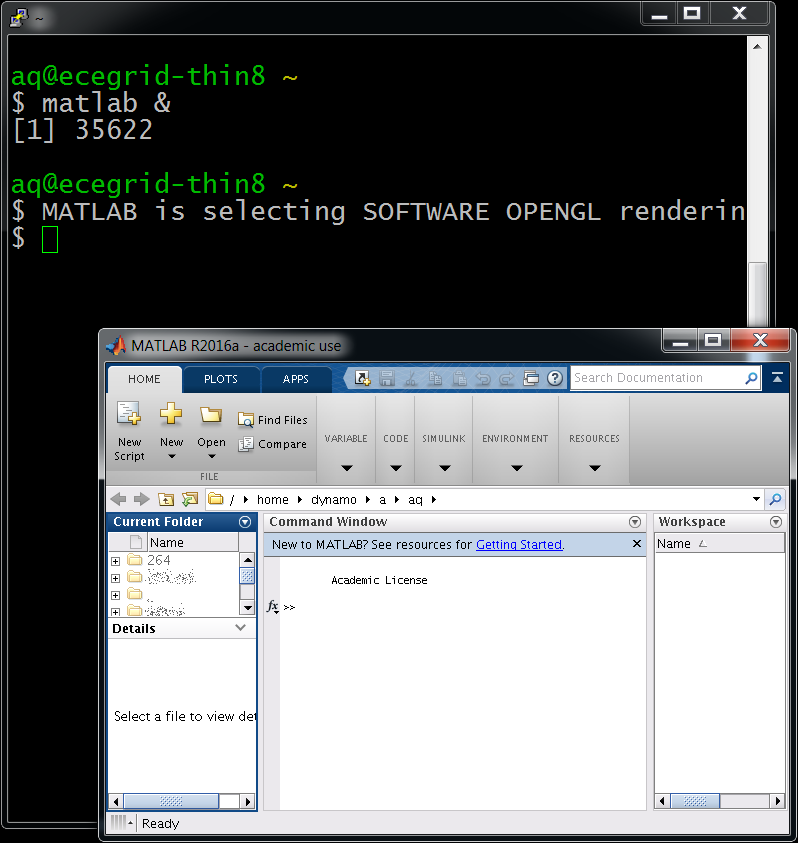 If you get any errors about the DISPLAY variable, make sure you did the setup properly.
 - [Windows/Mac/Linux] Install ThinLinc and connect to ecegrid.ecn.purdue.edu via ThinLinc. That will open a complete Linux desktop. It seems to work for most people, but some have had some issues with it.
- [Windows/Mac/Linux] If you have MATLAB installed, use sftp or scp to download the files to your computer.
- [Windows] Use WinSCP (graphical) or sftp (command line, included with PuTTY) to connect to ecegrid.ecn.purdue.edu..
- [Mac/Linux] Use the command line sftp or your favorite graphical sftp program.
- [Windows] Install Xming. It will run in the background. Then, from PuTTY, run
Updates
| 9/17/2017 | Added Q1 to Q&A about running MATLAB remotely. |