ME 200 – Thermodynamics I – Spring 2020
Homework 36: Vapor Compression Cycles with Superheat
Part (i): Expansion Valve
Part (ii): Turbine
Part (i): Expansion Valve
Given:
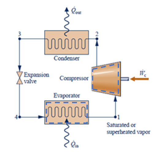
A standard 4-component vapor-compression cycle using R-134a is shown in the figure. The cycle is used as a refrigeration cycle to cool a refrigerator at 5 °C with a cooling capacity of 200 W, with a heat transfer to a kitchen at 20 °C. Assume that the pressure drops in the evaporator and condenser are negligible, and that the compressor and expansion valve are adiabatic. Take the boundary temperature for heat transfer into the evaporator to be 5 °C, and the boundary temperature for heat transfer out of the condenser to be 20 ºC. Assume the compressor suction state is $P_{1}$ = 2.4 bar and saturated vapor, the compressor discharge pressure is $P_{2}$ = 7.0 bar, the compressor isentropic efficiency is 70%, and the condenser outlet state is saturated liquid.
#Given Inputs:

import CoolProp.CoolProp as CP
CP.set_reference_state('R134a','ASHRAE')
from tabulate import tabulate

Q_dot_cool = 200                            # cooling capacity [W]

T_L = 5                                     # refrigerator (source) air temperature [ºC]
T_L_abs = T_L + 273.15                      # refrigerator air temperature [K]

T_H = 20                                    # kitchen (sink) air temperature [ºC]
T_L_abs = T_H + 273.15                      # kitchen air temperature [K]

P_1 = 2.4                                   # compressor suction pressure [bar]
P_2 = 7.0                                   # compressor discharge pressure [bar]

eta_c = 0.7                                 # compressor adiabatic isentropic efficiency [-]
Find:
a) mass flow rate of the cycle (g/s)
b) compressor input power (W)
c) compressor discharge temperature (ºC)
d) COP of the cycle
System Diagram:
Assumptions:
1) open system, 2) steady state, steady flow (SSSF), 3) adiabatic compressor and expansion valve, 4) negligible changes in kinetic and potential energy, 5) no work in the condenser and evaporator,
Basic Equations:
$$\dfrac{dm}{dt}=\Sigma \dot m_{in}-\Sigma \dot m_{out}$$$$\dfrac{dE}{dt} = \dot Q- \dot W + \displaystyle\sum_{in} \dot m_{in} (h+ke+pe)_{in}-\displaystyle\sum_{out} \dot m_{out}(h+ke+pe)_{out}$$$$\eta_{c} = \dfrac{w_{s}}{w_{act}}$$$$\dfrac{dS}{dt} = \displaystyle\sum \frac{\dot Q}{T_{b}} + \displaystyle\sum_{in} \dot m_{in} (s)_{in}-\displaystyle\sum_{out} \dot m_{out}(s)_{out}$$$$ COP_R = \dfrac{Q_C}{W_{net,in}}$$Solution:
The first step is to evaluate the properties at each state and put them in a state table. The following state table provides the known and unknown properties for temperature (T), pressure (P), enthalpy (h), entropy (s), and quality.
| State | T ($^{\circ}$C) | P (kPa) | h (kJ/kg) | s (kJ/kg-K) | Quality |
|---|---|---|---|---|---|
| 1 | 240 | 1 | |||
| 2 | 700 | - | |||
| 2s | 700 | - | |||
| 3 | 700 | 0 | |||
| 4 | 240 | - |
The provided data and tabular properties available on the ME 200 website were used to determine the unknown properties (temperature, enthalpies entropies qualities). The above table includes all of the actual states and the isentropic state exiting the compressor. We need the isentropic state in order to apply the compressor isentropic efficiency for determining the actual exit state. Unknown properties at states 1 and 3 can be determined using the SLVM pressure table for specified pressures and qualities. State 2s is a superheated vapor and the enthalpy and entropy properties were determined using the SHV tables. This required interpolation. State 4 was found in the SLVM tables using the enthalpy from state 3 since the valve is isenthalpic ($h_3=h_4$ since the valve is SSSF and adiabatic with negligible changes in ke and pe). This state is a two-phase mixture and given pressure and enthalpy can be used to determine the quality. Under the assumption of a SSSF and adiabatic compressor with negligible changes in kinetic and potential energy, then the compressor isentropic efficiency is used along with the enthalpies at states 1 and 2s to determine the enthalpy at state 2.
$$h_2 = h_1 + \dfrac{h_{2s} - h_1}{\eta _c}$$The resulting properties are shown in the table below.
| State | T ($^{\circ}$C) | P (kPa) | h (kJ/kg) | s (kJ/kg-K) | Quality |
|---|---|---|---|---|---|
| 1 | -5.37 | 240 | 247.3 | 0.93465 | 1 |
| 2 | 40.40 | 700 | 279.0 | 0.96543 | - |
| 2s | 30.99 | 700 | 269.5 | 0.93465 | - |
| 3 | 26.71 | 700 | 88.8 | 0.3324 | 0 |
| 4 | -5.37 | 240 | 88.8 | 0.34295 | 0.218 |
We can then use these properties to evaluate the other cycle performance parameters. Mass balances for each component are simplified using the assumption of steady flow ($dm/dt$=0) and a single inlet and outlet.
$$\dot m_{in}=\dot m_{out}=\dot m$$Energy balances are performed on the evaporator and compressor to determine the required mass flow rate for the specified cooling rate and input power to the compressor. The energy balances are simplified using the assumptions of steady state ($dE/dt$=0), negligible kinetic and potential energy changes, adiabatic compressor, and no work in the evaportaor.
Evaporator:
$$\dot Q_{cool} = \dot m (h_1-h_4)$$$$\dot m = \dot Q_{cool}/(h_1-h_4)$$Compressor:
$$\dot W_{comp} = \dot m (h_2-h_1)$$Cycle Performance
The coefficient of performance is the ratio of cooling provided to net work input. For the simple vapor compressor cycle, the net work input is just the compressor work. Therefore,
$$ COP_R = \dfrac{\dot Q_{cool}}{\dot W_{comp}}=\dfrac{h_1-h_4}{h_2-h_1}$$The following code window determines properties from an external python routine and calculates the cycle parameters necessary for this problem.
h_1 = CP.PropsSI('H','Q',1,'P',P_1*100000,'R134a')/1000            # compressor suction specific enthalpy [kJ/kg]
s_1 = CP.PropsSI('S','Q',1,'P',P_1*100000,'R134a')/1000            # compressor suction specific entropy [kJ/(kg-K)
T_1 = CP.PropsSI('T','Q',1,'P',P_1*100000,'R134a') - 273.15        # compressor suction temperature [ºC]
X_1 = CP.PropsSI('Q','H',h_1*1000,'P',P_1*100000,'R134a')          # compressor suction quality

h_2s = CP.PropsSI('H','S',s_1*1000,'P',P_2*100000,'R134a')/1000    # isentropic compression discharge specific enthalpy [kJ/kg]
T_2s = CP.PropsSI('T','S',s_1*1000,'P',P_2*100000,'R134a')-273.15  # isentropic compression discharge temperature [ºC]

h_2 = (h_1 + (h_2s - h_1)/eta_c)                                   # compressor discharge specific enthalpy [kJ/kg]
T_2 = CP.PropsSI('T','H',h_2*1000,'P',P_2*100000,'R134a') - 273.15 # compressor discharge temperature [ºC]
s_2 = CP.PropsSI('S','H',h_2*1000,'P',P_2*100000,'R134a')/1000     # compressor discharge specific entropy [kJ/(kg-K)]

h_3 = CP.PropsSI('H','Q',0,'P',P_2*100000,'R134a')/1000            # condenser outlet specific enthalpy [kJ/kg]
s_3 = CP.PropsSI('S','Q',0,'P',P_2*100000,'R134a')/1000            # condenser outlet specific entropy [kJ/(kg-K)]
T_3 = CP.PropsSI('T','H',h_3*1000,'P',P_2*100000,'R134a') - 273.15 # condenser discharge temperature [ºC]
X_3 = CP.PropsSI('Q','H',h_3*1000,'P',P_2*100000,'R134a')          # condenser discharge quality

h_4 = h_3                                                          # evaporator inlet specific enthalpy [kJ/kg]
T_4 = CP.PropsSI('T','H',h_4*1000,'P',P_1*100000,'R134a') - 273.15 # evaporator inlet temperature [ºC]
s_4 = CP.PropsSI('S','H',h_4*1000,'P',P_1*100000,'R134a')/1000     # evaporator inlet specific entropy [kJ/(kg-K)]
X_4 = CP.PropsSI('Q','H',h_4*1000,'P',P_1*100000,'R134a')          # evaporator inlet quality

m_dot = Q_dot_cool/(h_1 - h_4)                                     # system mass flow rate [g/s]

W_dot_comp = m_dot*(h_2 - h_1)                                     # compressor power consumption [W]

COP = (h_1 - h_4)/(h_2 - h_1)                                      # cycle COP [-]

myData = [("1",P_1*100,T_1,X_1,h_1,s_1),("2",P_2*100,T_2,"-",h_2,s_2),("2s",P_2*100,T_2s,"-",h_2s,s_1),
          ("3",P_2*100,T_3,X_3,h_3,s_3),("4",P_1*100,T_4,round(X_4,4),h_4,s_4)]

headers = ["State","P(kPa)","T(C)","X(-)","h(kJ/kg)","s(kJ/kg-K)"]
print(tabulate(myData,headers=headers,tablefmt="fancy_grid",floatfmt=(".0f",".0f","0.1f","0.3f","0.1f","0.5f")))

print('Mass flow rate =',round(m_dot,3),'[g/s]')
print('Compressor input power =',round(W_dot_comp,2),'[W]')
print('Compressor discharge temperature =',round(T_2,2),'[deg C]')
print('COP =',round(COP,2),'[-]')
#Given Inputs:
eta_t = 0.7                          # turbine adiabatic isentropic efficiency [-]
System Diagram:
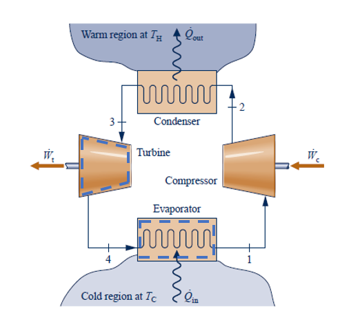
Changes in Assumptions:
1) adiabatic turbine replaces adiabatic valve
Additional Basic Equation:
$$\eta_{t} = \dfrac{w_{act}}{w_{s}}$$Solution:
The first step is to evaluate the properties at each state and put them in a state table. The following state table provides the known and unknown properties for temperature (T), pressure (P), enthalpy (h), entropy (s), and quality. All of the properties from part (i) that didn't change were inherited in this table. In addition, state 4 is replaced with state 4t to denote that this state is different than for part (i).
| State | T ($^{\circ}$C) | P (kPa) | h (kJ/kg) | s (kJ/kg-K) | Quality |
|---|---|---|---|---|---|
| 1 | -5.37 | 240 | 247.3 | 0.93465 | 1 |
| 2 | 40.40 | 700 | 279.0 | 0.96543 | - |
| 2s | 30.99 | 700 | 269.5 | 0.93465 | - |
| 3 | 26.71 | 700 | 88.8 | 0.3324 | 0 |
| 4t | 240 | - | |||
| 4s | 240 | - |
The above table includes both the actual and isentropic states leaving the turbine. We need the isentropic state in order to apply the turbine isentropic efficiency for determining the actual exit state. Under the assumption of a SSSF and adiabatic turbine with negligible changes in kinetic and potential energy, then the turbine isentropic efficiency is used along with the enthalpies at states 3 and 4s to determine the enthalpy at state 4t.
$$h_{4t} = h_3 - \eta _t (h_3 - h_{4s})$$The resulting properties are shown in the table below.
| State | T ($^{\circ}$C) | P (kPa) | h (kJ/kg) | s (kJ/kg-K) | Quality |
|---|---|---|---|---|---|
| 1 | -5.37 | 240 | 247.3 | 0.93465 | 1 |
| 2 | 40.40 | 700 | 279.0 | 0.96543 | - |
| 2s | 30.99 | 700 | 269.5 | 0.93465 | - |
| 3 | 26.71 | 700 | 88.8 | 0.3324 | 0 |
| 4t | -5.37 | 240 | 86.83 | 0.34295 | 0.208 |
| 4s | -5.37 | 240 | 86.02 | 0.3324 | 0.204 |
The analysis of the evaporator is the same as part (i), but the inlet state (4t) is different. Therefore,
$$\dot Q_{cool}= \dot m(h_1-h_{4t})$$and the required flow rate is
$$\dot m = \dot Q_{cool}/(h_1-h_{4t})$$An energy balance on the turbine (SSSF, adiabatic, $\Delta ke = \Delta pe = 0$) gives the following for the turbine power output.
$$\dot W_{t} = \dot m (h_3-h_{4t})$$This turbine power output can be used to help drive the compressor (they could be on the same rotating shaft), such that the net required power input is difference between compressor and turbine power.
$$\dot W_{net,in} = \dot W_{c} - \dot W_{t}$$Then, the overall cycle COP can be expressed as
$$ COP_R = \dfrac{\dot Q_{cool}}{\dot W_{c} - \dot W_{t}} = \dfrac{h_1 - h_{4t}}{(h_2 - h_1)-(h_3 - h_{4t})}$$The following code window determines the unknown properties from an external python routine and calculates the updated cycle parameters for this problem.
h_4_s = CP.PropsSI('H','S',s_3*1000,'P',P_1*100000,'R134a')/1000       # isentropic turbine outlet specific enthalpy [kJ/kg]
X_4_s = CP.PropsSI('Q','S',s_3*1000,'P',P_1*100000,'R134a')            # isentropic turbine outlet quality

h_4_t = h_3 - (h_3 - h_4_s)*eta_t                                      # actual turbine outlet specific enthalpy [kJ/kg]
s_4_t = CP.PropsSI('S','H',h_4_t*1000,'P',P_1*100000,'R134a')/1000     # actual turbine outlet specific entropy [kJ/(kg-K)]
X_4_t = CP.PropsSI('Q','H',h_4_t*1000,'P',P_1*100000,'R134a')          # actual turbine outlet quality

m_dot_t = Q_dot_cool/(h_1 - h_4_t)                                     # system mass flow rate with turbine [g/s]

COP_t = (h_1 - h_4_t)/((h_2 - h_1) - (h_3 - h_4_t))                    # cycle COP with turbine [-]

myData = [("1",P_1*100,T_1,X_1,h_1,s_1),("2",P_2*100,T_2,"-",h_2,s_2),("2s",P_2*100,T_2s,"-",h_2s,s_1),
          ("3",P_2*100,T_3,X_3,h_3,s_3),("4t",P_1*100,T_4,round(X_4_t,3),h_4_t,s_4_t),("4s",P_1*100,T_4,round(X_4_s,3),h_4_s,s_3)]

headers = ["State","P(kPa)","T(C)","X(-)","h(kJ/kg)","s(kJ/kg-K)"]
print(tabulate(myData,headers=headers,tablefmt="fancy_grid",floatfmt=(".0f",".0f","0.1f","0.3f","0.1f","0.5f")))

print('mass flow rate with the turbine =',round(m_dot_t,3),'[g/s]')
print('cycle COP with the turbine =',round(COP_t,2),'[-]')