Given:
A Rankine cycle with reheat. Steam leaves the low pressure turbine at 500 kPa and is reheated to 520 C. Both turbine stages have an isentropic efficiency of 81.3%.
#Given Inputs:
P_1 = 0.08*100      # pressure at state 1 [kPa]
P_2 = 100*100       # pressure at state 2 [kPa]
P_3 = 100*100       # pressure at state 3 [kPa]
P_4 = 100*100       # pressure at state 4 [kPa]
P_5 = 5*100         # pressure at state 5 [kPa]
P_5i = 5*100        # pressure of state 5' [kPa]
P_5ii = 0.08*100    # pressure of state 5'' [kPa]
T_2 = 43+273.15     # temperature at state 2 [K]
T_4 = 520+273.15    # temperature at state 4 [K]
T_5i = 520+273.15   # temperature of state 5' [K]
X_1 = 0.0           # quality at state 1
X_3 = 1.0           # quality at state 3
eta_t = 0.813       # efficiency of the turbine stages
Find:
The net work output per unit mass and the thermal efficiency. Compare the results to HW 34.
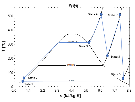
Sketch a T-s diagram
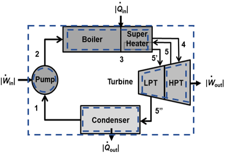
System Diagram:
The system is made up of the individual components of the Rankine cycle. Each component is evaluated individually and then the system can be evaluated as a whole.
Assumptions:
1) open system, 2) steady state, steady flow (SSSF) 3) adiabatic for pump, turbine, and exterior shell of the condenser, 4) negligible changes in kinetic and potential energy, 5) uniform properties at all states
Basic Equations:
$$\dfrac{dm}{dt}=\Sigma \dot m_{in}-\Sigma \dot m_{out}$$$$\dfrac{dE}{dt} = \dot Q- \dot W + \displaystyle\sum_{in} \dot m_{in} (h+ke+pe)_{in}-\displaystyle\sum_{out} \dot m_{out}(h+ke+pe)_{out}$$$$\dfrac{dS}{dt} = \displaystyle\sum_{j} \dfrac{\dot Q_j}{T_{j,boundary}}+ \displaystyle\sum_{in} \dot m_{in} s_{in}-\displaystyle\sum_{out} \dot m_{out}s_{out}+\dot \sigma _{generation}$$$$\eta _{th} = \dfrac{W_{net}}{Q_{in}}, \eta _t = \dfrac{W_{act}}{W_s}$$Solution:
The first step is to evaluate the properties at each state and put them in a state table. The following state table provides the known and unknown properties for temperature (T), pressure (P), enthalpy (h), entropy (s), and quality.
| State | T ($^{\circ}$C) | P (kPa) | h (kJ/kg) | s (kJ/kg-K) | Quality |
|---|---|---|---|---|---|
| 1 | 8 | 173.84 | 0.59249 | 0 | |
| 2 | 43 | 10000 | 188.854 | 0.60605 | - |
| 3 | 10000 | 1 | |||
| 4 | 520 | 10000 | 3426.4 | 6.6649 | - |
| 5 | 500 | ||||
| 5s | 500 | ||||
| 5' | 520 | 500 | |||
| 5'' | 8 | ||||
| 5''s | 8 |
The provided data for enthalpies and entropies in this table were determined using tabular data available on the ME 200 website. The above table includes all of the actual states and the isentropic states for the exits of the turbine (5s and 5''s). We need the isentropic states in order to apply the turbine isentropic efficiency for determining the actual exit states. Unknown properties at states 1 and 3 can be determined using the SLVM pressure table for specified pressures and qualities. State 2 is a compressed liquid at high pressure and the enthalpy and entropy properties were determined using the CL tables. This required interpolation. State 4 was found in the SHV tables. For states 5s and 5''s, we need to evaluate $h_{5s}$ at $P_5$ and $s_5=s_4$ and $h_{5''s}$ at $P_5''$ and $s_5''=s_5'$ . These states are both a two-phase mixture requiring determination of quality ($x_{5s}$ and $x_{5''s}$).
In order to determine the exit enthalpy for each turbine stage, we apply the definition for turbine isentropic efficiency and employ the assumptions that the process are adiabatic with negligigle changes in kinetic and potential energy. Then,
$$\eta _t = \dfrac{w_{act}}{w_s} = \dfrac{h_4-h_5}{h_4-h_{5s}} = \dfrac{h_4-h_5}{h_4-h_{5s}}$$Therefore,
$$h_5 = h_4 - \eta _t (h_4-h_{5s})$$$$h_5'' = h_{5'} - \eta _t (h_{5'}-h_{5''s})$$The completed table based on the properties on the ME 200 website is as follows.
| State | T ($^{\circ}$C) | P (kPa) | h (kJ/kg) | s (kJ/kg-K) | Quality |
|---|---|---|---|---|---|
| 1 | 41.51 | 8 | 173.84 | 0.59249 | 0 |
| 2 | 43 | 10000 | 188.854 | 0.60605 | - |
| 3 | 311.0 | 10000 | 2725.5 | 5.6160 | 1 |
| 4 | 520 | 10000 | 3426.4 | 6.6649 | - |
| 5 | 184.0 | 500 | 2821.1 | 6.9864 | - |
| 5s | 151.83 | 500 | 2681.9 | 6.6649 | 0.9686 |
| 5' | 520 | 500 | 3528.1 | 8.1422 | - |
| 5'' | 41.51 | 8 | 2732.4 | 8.6697 | - |
| 5''s | 41.51 | 8 | 2549.4 | 8.1422 | 0.9889 |
Alternatively, we could use public-domain property routines available in Python (CoolProp) to evalute all of the properties as follows.
import CoolProp.CoolProp as CP
import numpy as np
from tabulate import tabulate

h_1 = CP.PropsSI('H','P',P_1*1000,'Q',X_1,'Water')/1000.         # enthalpy of water at state 1 [kJ/kg]
s_1 = CP.PropsSI('S','P',P_1*1000,'Q',X_1,'Water')/1000.         # entropy of water at state 1 [kJ/kgK]
T_1 = CP.PropsSI('T','P',P_1*1000,'Q',X_1,'Water')               # temperature of water at state 1 [K]

h_2 = CP.PropsSI('H','P',P_2*1000,'T',T_2,'Water')/1000.         # enthalpy of water at state 2 [kJ/kg]
s_2 = CP.PropsSI('S','P',P_2*1000,'T',T_2,'Water')/1000.         # entropy of water at state 2 [kJ/kgK]

h_3 = CP.PropsSI('H','P',P_3*1000,'Q',X_3,'Water')/1000.         # enthalpy of water at state 3 [kJ/kg]
s_3 = CP.PropsSI('S','P',P_3*1000,'Q',X_3,'Water')/1000.         # entropy of water at state 3 [kJ/kgK]
T_3 = CP.PropsSI('T','P',P_3*1000,'Q',X_3,'Water')               # temperature of water at state 3 [K]

h_4 = CP.PropsSI('H','P',P_4*1000,'T',T_4,'Water')/1000.         # enthalpy of water at state 4 [kJ/kg]
s_4 = CP.PropsSI('S','P',P_4*1000,'T',T_4,'Water')/1000.         # entropy of water at state 4 [kJ/kgK]

s_5s = s_4
h_5s = CP.PropsSI('H','P',P_5*1000,'S',s_5s*1000,'Water')/1000.  # enthalpy of water at state 5s [kJ/kg]
T_5s = CP.PropsSI('T','P',P_5*1000,'H',h_5s*1000.,'Water')       # temperature of water at state 5s [K]
X_5s = CP.PropsSI('Q','P',P_5*1000,'H',h_5s*1000.,'Water')       # quality of water at state 5s [K]
X_5s = round(X_5s,3)

h_5 = h_4 - eta_t*(h_4-h_5s)                                     # enthalpy of water at state 5 [kJ/kg]
s_5 = CP.PropsSI('S','P',P_5*1000,'H',h_5*1000,'Water')/1000.    # entropy of water at state 5 [kJ/kgK]
T_5 = CP.PropsSI('T','P',P_5*1000,'H',h_5*1000,'Water')          # temperature of water at state 5 [K]

h_5i = CP.PropsSI('H','P',P_5i*1000,'T',T_5i,'Water')/1000.      # enthalpy of water at state 5' [kJ/kg]
s_5i = CP.PropsSI('S','P',P_5i*1000,'T',T_5i,'Water')/1000.      # entropy of water at state 5' [kJ/kgK]

s_5sii = s_5i
T_5sii = CP.PropsSI('T','P',P_5ii*1000,'S',s_5sii*1000,'Water')        # temperature of water at state 5s''[K]
h_5sii = CP.PropsSI('H','P',P_5ii*1000,'S',s_5sii*1000,'Water')/1000.  # enthalpy of water at state 5s'' [kJ/kg]
X_5sii = CP.PropsSI('Q','P',P_5ii*1000,'H',h_5sii*1000.,'Water')       # quality of water at state 5s'' [K]
X_5sii = round(X_5sii,3)

h_5ii = h_5i - eta_t*(h_5i-h_5sii)                                   # enthalpy of water at state 5'' [kJ/kg]
s_5ii = CP.PropsSI('S','P',P_5ii*1000,'H',h_5ii*1000,'Water')/1000.  # entropy of water at state 5'' [kJ/kgK]
T_5ii = CP.PropsSI('T','P',P_5ii*1000,'H',h_5ii*1000,'Water')        # temperature of water at state 5'' [K]
X_5ii = CP.PropsSI('Q','P',P_5ii*1000,'H',h_5ii*1000.,'Water')       # quality of water at state 5'' [K]
X_5ii = round(X_5ii,3)

MyData = [("1",P_1,T_1-273.15,X_1,h_1,s_1),           ("2",P_2,T_2-273.15,"-",h_2,s_2),
          ("3",P_3,T_3-273.15,X_3,h_3,s_3),           ("4",P_4,T_4-273.15,"-",h_4,s_4),
          ("5s",P_5,T_5s-273.15,X_5s,h_5s,s_4),       ("5",P_5,T_5-273.15,'-',h_5,s_5),
          ("5i",P_5i,T_5i-273.15,"-",h_5i,s_5i),      ("5sii",P_5ii,T_5sii-273.15,X_5sii,h_5sii,s_5sii),
          ("5ii",P_5ii,T_5ii-273.15,"-",h_5ii,s_5ii)]

headers = ["State","P(kPa)","T(C)","X(-)","h(kJ/kg)","s(kJ/kg-K)"]
print(tabulate(MyData,headers=headers,tablefmt="fancy_grid",floatfmt=(".0f",".0f","0.1f","0.3f","0.1f","0.5f")))
There are some slight differences in properties, but they will have negligible effect on the final results.
At this point, all of the necessary are available to solve the problem. A mass balance is applied to each flow stream with the assumption of steady flow ($dm/dt=0$).
$$\dot m_{5''} = \dot m_{5'} = \dot m_{5} = \dot m_{4} = \dot m_{3} = \dot m_{2} = \dot m_{1} = \dot m_{cycle}$$An energy balance is applied to each component of the system with the assumption of SSSF ($dE/dt=0$), negligible change in potential and kinetic energy, and adiabatic pumps and turbines. The simplified energy balances:
High pressure turbine: $w_{45}=h_4-h_5$
Low pressure turbine: $w_{5'5''}=h_{5'}-h_{5''}$
Pump: $w_{12}=h_1-h_2$
Boiler: $q_{24}=h_4-h_2$
Reheat: $q_{55'}=h_{5'}-h_{5}$
The net work output of the cycle per unit mass of flow is the sum of the work for the high stage turbine, low stage turbine, and pump
$$w_{net}=w_{45}+w_{5'5''}+w_{12}$$The total heat transfer into the system is the sum of the heat transfer for the boiler and reheat.
$$q_{in}=q_{24}+q_{55'}=h_4-h_2+h_{5'}-h_{5}$$The overall system efficiency is
$$\eta _{th} = \dfrac{w_{net}}{q_{in}}$$w_45 = h_4 - h_5 # high pressure turbine work output [kJ/kg]
w_5i5ii = h_5i - h_5ii # low pressure turbine work output [kJ/kg]
w_12 = h_1 - h_2 # pump work input [kJ/kg]
w_net = w_45 + w_5i5ii + w_12 # net cycle work output per unit mass of flow [kJ/kg]
q_24 = h_4 - h_2 # boiler heat input [kJ/kg]
q_55i = h_5i - h_5 # reheat inoput [kJ/kg]
q_in = (h_4-h_2)+(h_5i-h_5) # total heat input per unit mass of flow [kJ/kg]
eta_th = w_net/q_in # overall cycle efficiency
print('w_45 = ',round(w_45,1),'kJ/kg')
print('w_5i5ii = ',round(w_5i5ii,1),'kJ/kg')
print('w_12 = ',round(w_12,1),'kJ/kg')
print('q_in = ',round(q_in,1),'kJ/kg')
print('w_net = ',round(w_net,1),'kJ/kg')
print('eta_th = ',round(eta_th,3))
The work output and the efficiency of the cycle are higher than for HW34. The reheat cycle is more effective because of the higher average temperature for heat transfer to the cycle.