Given:
A Rankine cycle with a superheated vapor at the boiler exit (turbine inlet). The cycle produces 120 MW of net power with water/steam as the working fluid.
#Given Inputs:
P_1 = 0.08*100      # pressure at state 1 [kPa]
P_2 = 100*100       # pressure at state 2 [kPa]
P_3 = 100*100       # pressure at state 3 [kPa]
P_4 = 100*100       # pressure at state 4 [kPa]
P_5 = 0.08*100      # pressure at state 5 [kPa]
P_6 = 1*100         # pressure at state 6 [kPa]
P_7 = 1*100         # pressure at state 7 [kPa]
T_2 = 43+273.15     # temperature at state 2 [K]
T_4 = 520+273.15    # temperature at state 4 [K]
T_6 = 20+273.15     # temperature at state 6 [K]
T_7 = 35+273.15     # temperature at state 7 [K]
X_1 = 0.0           # quality at state 1
X_3 = 1.0           # quality at state 3
X_5 = 0.9           # quality of state 5
W_dot_net = 120000  # net power output from cycle [kW]
Find:
(a) mass flow of water (steam) in the cycle, in kg/s
(b) thermal efficiency of the cycle
(c) isentropic turbine efficiency
(d) mass flow rate of the cooling water in the condenser, in kg/s
(e) rates of entropy production, each in kW/K, for the turbine, condenser, and pump
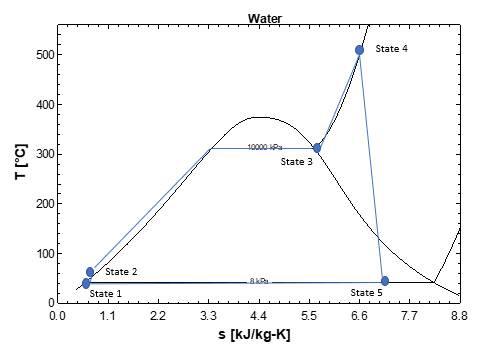
Sketch a T-s diagram.
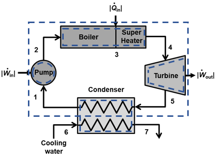
System Diagram:
The system is made up of the individual components of the Rankine cycle. Each component is evaluated individually along with the system as a whole.
Assumptions:
1) open system, 2) steady state, steady flow (SSSF) 3) adiabatic for pump, turbine, and exterior shell of the condenser, 4) negligible changes in kinetic and potential energy, 5) uniform properties at all states
Basic Equations:
$$\dfrac{dm}{dt}=\Sigma \dot m_{in}-\Sigma \dot m_{out}$$$$\dfrac{dE}{dt} = \dot Q- \dot W + \displaystyle\sum_{in} \dot m_{in} (h+ke+pe)_{in}-\displaystyle\sum_{out} \dot m_{out}(h+ke+pe)_{out}$$$$\dfrac{dS}{dt} = \displaystyle\sum_{j} \dfrac{\dot Q_j}{T_{j,boundary}}+ \displaystyle\sum_{in} \dot m_{in} s_{in}-\displaystyle\sum_{out} \dot m_{out}s_{out}+\dot \sigma _{generation}$$$$\eta _{th} = \dfrac{\dot W_{net}}{\dot Q_{in}}, \eta _t = \dfrac{w_{act}}{w_s}$$Solution:
The first step is to evaluate the properties at each state and put them in a state table. The following state table provides the known and unknown properties for temperature (T), pressure (P), enthalpy (h), entropy (s), and quality.
| State | T ($^{\circ}$C) | P (kPa) | h (kJ/kg) | s (kJ/kg-K) | Quality |
|---|---|---|---|---|---|
| 1 | 8 | 173.84 | 0.59249 | 0.0 | |
| 2 | 43 | 10000 | 188.854 | 0.60605 | - |
| 3 | 10000 | 1.0 | |||
| 4 | 520 | 10000 | 3426.4 | 6.6649 | - |
| 5 | 8 | 0.9 | |||
| 5s | 8 | ||||
| 6 | 20 | 100 | 84.01 | 0.29648 | - |
| 7 | 35 | 100 | 146.72 | 0.50513 | - |
The provided data for enthalpies and entropies in this table were determined using tabular data available on the ME 200 website. The above table includes all of the actual states and the isentropic state for the exit of the turbine (5s). We need state 5s in order to determine the isentropic efficiency of the turbine. Unknown properties at states 1, 3, and 5 can be determined using the SLVM pressure table for specified pressures and qualities. State 2 is a compressed liquid at high pressure and the enthalpy and entropy properties were determined using the CL tables. This required interpolation. State 4 was found in the SHV tables. For state 5s, we need to evaluate $h_{5s}$ at $P_5$ and $s_5=s_4$. This state is a two-phase mixture and we can determine a quality ($x_{5s}$).
The completed table based on the properties on the ME 200 website is as follows.
| State | T ($^{\circ}$C) | P (kPa) | h (kJ/kg) | s (kJ/kg-K) | Quality |
|---|---|---|---|---|---|
| 1 | 41.51 | 8 | 173.84 | 0.59249 | 0.0 |
| 2 | 43 | 10000 | 188.854 | 0.60605 | - |
| 2s | 41.8 | 10000 | 184.34 | 0.59249 | - |
| 3 | 311.0 | 10000 | 2725.5 | 5.6160 | 1.0 |
| 4 | 520 | 10000 | 3426.4 | 6.6649 | - |
| 5 | 41.51 | 8 | 2336.0 | 7.4638 | 0.9 |
| 5s | 41.51 | 8 | 2084.7 | 6.6649 | 0.795 |
| 6 | 20 | 100 | 84.01 | 0.29648 | - |
| 7 | 35 | 100 | 146.72 | 0.50513 | - |
Alternatively, we could use public-domain property routines available in Python (CoolProp) to evalute all of the properties as follows.
import CoolProp.CoolProp as CP
import numpy as np
from tabulate import tabulate

h_1 = CP.PropsSI('H','P',P_1*1000,'Q',X_1,'Water')/1000.         # enthalpy of water at state 1 [kJ/kg]
s_1 = CP.PropsSI('S','P',P_1*1000,'Q',X_1,'Water')/1000.         # entropy of water at state 1 [kJ/kgK]
T_1 = CP.PropsSI('T','P',P_1*1000,'Q',X_1,'Water')               # temperature of water at state 1 [K]

h_2 = CP.PropsSI('H','P',P_2*1000,'T',T_2,'Water')/1000.         # enthalpy of water at state 2 [kJ/kg]
s_2 = CP.PropsSI('S','P',P_2*1000,'T',T_2,'Water')/1000.         # entropy of water at state 2 [kJ/kgK]

h_3 = CP.PropsSI('H','P',P_3*1000,'Q',X_3,'Water')/1000.         # enthalpy of water at state 3 [kJ/kg]
s_3 = CP.PropsSI('S','P',P_3*1000,'Q',X_3,'Water')/1000.         # entropy of water at state 3 [kJ/kgK]
T_3 = CP.PropsSI('T','P',P_3*1000,'Q',X_3,'Water')               # temperature of water at state 3 [K]

h_4 = CP.PropsSI('H','P',P_4*1000,'T',T_4,'Water')/1000.         # enthalpy of water at state 4 [kJ/kg]
s_4 = CP.PropsSI('S','P',P_4*1000,'T',T_4,'Water')/1000.         # entropy of water at state 4 [kJ/kgK]

h_5 = CP.PropsSI('H','P',P_5*1000,'Q',X_5,'Water')/1000.         # enthalpy of water at state 5 [kJ/kg]
s_5 = CP.PropsSI('S','P',P_5*1000,'Q',X_5,'Water')/1000.         # entropy of water at state 5 [kJ/kgK]
T_5 = CP.PropsSI('T','P',P_5*1000,'Q',X_5,'Water')               # temperature of water at state 5 [K]

s_5s = s_4
h_5s = CP.PropsSI('H','P',P_5*1000,'S',s_5s*1000,'Water')/1000.  # enthalpy of water at state 5s [kJ/kg]
T_5s = CP.PropsSI('T','P',P_5*1000,'H',h_5s*1000.,'Water')       # temperature of water at state 5s [K]
X_5s = CP.PropsSI('Q','P',P_5*1000,'H',h_5s*1000.,'Water')       # quality of water at state 5s [K]
X_5s = round(X_5s,3)

h_6 = CP.PropsSI('H','P',P_6*1000,'T',T_6,'Water')/1000.         # enthalpy of water at state 6 [kJ/kg]
s_6 = CP.PropsSI('S','P',P_6*1000,'T',T_6,'Water')/1000.         # entropy of water at state 6 [kJ/kgK]

h_7 = CP.PropsSI('H','P',P_7*1000,'T',T_7,'Water')/1000.         # enthalpy of water at state 7 [kJ/kg]
s_7 = CP.PropsSI('S','P',P_7*1000,'T',T_7,'Water')/1000.         # entropy of water at state 7 [kJ/kgK]

myData = [("1",P_1,T_1-273.15,X_1,h_1,s_1), ("2",P_2,T_2-273.15,"-",h_2,s_2),
          ("3",P_3,T_3-273.15,X_3,h_3,s_3), ("4",P_4,T_4-273.15,"-",h_4,s_4),
          ("5",P_5,T_5-273.15,X_5,h_5,s_5), ("5s",P_5,T_5s-273.15,X_5s,h_5s,s_4),
          ("6",P_6,T_6-273.15,"-",h_6,s_6), ("7",P_7,T_7-273.15,"-",h_7,s_7)]

headers = ["State","P(kPa)","T(C)","X(-)","h(kJ/kg)","s(kJ/kg-K)"]
print(tabulate(myData,headers=headers,tablefmt="fancy_grid",floatfmt=(".0f",".0f","0.1f","0.3f","0.1f","0.5f")))
The properties are exactly the same except for slight differences in enthalpy values for compressed liquid states (states 2, 6, and 7). This could be due to linear interpolation for use of the tables. We will use the computer-generated data for the remainder of this solution, but will include two results for entropy generation for the pump based on the two different exit enthalpy values.
At this point, all of the necessary are available to solve the problem.
A mass balance is applied to each flow stream with the assumption of steady flow ($dm/dt=0$).
$$\dot m_{5} = \dot m_{4} = \dot m_{3} = \dot m_{2} = \dot m_{1} = \dot m_{cycle}$$$$\dot m_{7} = \dot m_{6} = \dot m_{cooling}$$An energy balance and an entropy balance are applied to each component of the system with the assumption of SSSF ($dS/dt=0=dE/dt$), negligible changes in potential and kinetic energy, and adiabatic pumps and turbines. The simplified energy and entropy balances become:
Turbine:
$$\dot W_{45}=\dot m_{cycle} (h_4-h_5)$$$$\dot \sigma_t = \dot m_{cycle} (s_5-s_4)$$Pump:
$$\dot W_{12}=\dot m_{cycle} (h_1-h_2)$$$$\dot \sigma_p = \dot m_{cycle} (s_2-s_1)$$Boiler:
$$ Q_{24}=\dot m_{cycle} (h_4-h_2)$$Condenser:
$$\dot m_{cooling}(h_6-h_7)=\dot m_{cycle}(h_1-h_5)$$$$\dot \sigma_c = \dot m_{cycle} (s_1-s_5)+\dot m_{cooling} (s_7-s_6)$$Part a)
The net power output of the cycle is given, but is also the sum of turbine and pump power determined from the energy balances.
$$\dot W_{net}=\dot W_{45} + \dot W_{12} = \dot m_{cycle} (h_4-h_5) + \dot m_{cycle} (h_1 - h_2)$$Solving for the mass flowrate:
$$\dot m_{cycle}= \dfrac {\dot W_{net}}{((h_4-h_5)+(h_1-h_2))}$$m_dot_cycle = W_dot_net/((h_4-h_5)+(h_1-h_2)) # water (steam) flow rate [kg/s]
print('m_dot_cycle = ',round(m_dot_cycle,2),'kg/s')
Part b)
The thermal efficiency of the cycle is
$$\eta_{th}=\dfrac{\dot W_{net}}{\dot Q_{in}}$$where
$$\dot Q_{in}=\dot Q_{24}=\dot m_{cycle} (h_4-h_2)$$Q_dot_in = m_dot_cycle*(h_4-h_2)
eta_th = np.abs((W_dot_net)/Q_dot_in)
print('W_dot_net = ',round(W_dot_net,5),'kW')
print('Q_dot_in = ',round(Q_dot_in,1),'kW')
print('eta_th = ',round(eta_th,3))
Part c)
The isentropic turbine efficiency is defined as
$$\eta _t = \dfrac{w_{act}}{w_s}$$where for an adiabatic turbine with negligible changes in kinetic and potential energy, this reduces to
$$\eta _t = \dfrac{h_4-h_5}{h_4-h_{5s}}$$eta_t = (h_4-h_5)/(h_4-h_5s)
print('eta_t = ',round(eta_t,3))
Part d)
The overall energy balance on the condenser can be used to determine the mass flow rate of the cooling water from the known cycle flow rate and properties.
$$\dot m_{cooling}(h_6-h_7)=\dot m_{cycle}(h_1-h_5)$$so that
$$\dot m_{cooling}=\dfrac{\dot m_{cycle}(h_1-h_5)}{(h_6-h_7)}$$m_dot_cooling = m_dot_cycle*(h_1-h_5)/(h_6-h_7)
print('m_dot_cooling = ',round(m_dot_cooling,1),'kg/s')
Part e)
Finally, the rates of entropy production for the turbine, condenser, and pump can be found from the entropy balances for each of these components.
$$\dot \sigma _c = \dot m_{cycle} (s_1-s_5)+\dot m_{cooling} (s_7-s_6)$$$$\dot \sigma _t = \dot m_{cycle} (s_5-s_4)$$$$\dot \sigma _p = \dot m_{cycle} (s_2-s_1)$$sigma_dot_c = m_dot_cycle*(s_1-s_5)+m_dot_cooling*(s_7-s_6)
sigma_dot_t = m_dot_cycle*(s_5-s_4)
sigma_dot_p = m_dot_cycle*(s_2-s_1)
s_2_tables = 0.60605 # from Blackboard properties [kJ/kg-K]
sigma_dot_p2 = m_dot_cycle*(s_2_tables-s_1)
print('sigma_dot_c = ',round(sigma_dot_c,2),'kW/K')
print('sigma_dot_t = ',round(sigma_dot_t,2),'kW/K')
print('sigma_dot_p = ',round(sigma_dot_p,2),'kW/K')
print('sigma_dot_p(table data) = ',round(sigma_dot_p2,2),'kW/K')