ME 200 – Thermodynamics I – Spring 2020
Homework 33: Rankine Cycles
Part (i): Ideal Rankine Cycle
Part (ii): Carnot Rankine Cycle
Part (iii): Rankine Cycle with Imperfect Turbine and Pump
All three parts use the same system diagram along with many of the same basic equations and assumptions. The common system, assumptions, and basic equations are given here with additional ones provided in the individual parts below.
System Diagram:
The system is made up of the individual components of the Rankine cycle. Each component is evaluated individually and then the system is evaluated as a whole.

Common Assumptions:
1) open system, 2) steady state, steady flow (SSSF) 3) adiabatic pump and turbine, 4) negligible changes in kinetic and potential energy, 5) uniform properties at states 1-4
Common Basic Equations:
$$\dfrac{dm}{dt}=\Sigma \dot m_{in}-\Sigma \dot m_{out}$$$$\dfrac{dE}{dt} = \dot Q- \dot W + \displaystyle\sum_{in} \dot m_{in} (h+ke+pe)_{in}-\displaystyle\sum_{out} \dot m_{out}(h+ke+pe)_{out}$$$$\eta _{th} = \dfrac{\dot W_{net}}{\dot Q_{in}}$$#Given Inputs:
P_1 = 0.02*100 # pump inlet pressure (low-side pressure) [kPa]
P_2 = 10*100 # pump outlet pressure (high-side pressure) [kPa]
P_3 = P_2 # turbine inlet pressure [kPa]
P_4 = P_1 # turbine outlet pressure [kPa]
X_1 = 0 # pump inlet quality
X_3 = 1 # turbine inlet quality
Find:
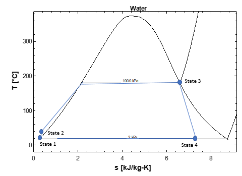
The net work output per unit mass of flow (kJ/kg) and the cycle efficiency. Sketch a Ts diagram for the cycle.
Additional Assumptions:
1) internally reversible processes
Additional Basic Equations:
None
Solution:
A first step can be to evaluate the properties at each state and put them in a state table. This can really help in keeping the process and solution organized. The following state table provides the known and unknown properties for temperature (T), pressure (P), enthalpy (h), entropy (s), and quality.
| State | T ($^{\circ}$C) | P (kPa) | h (kJ/kg) | s (kJ/kg-K) | Quality |
|---|---|---|---|---|---|
| 1 | 2 | 0 | |||
| 2 | 1000 | ||||
| 3 | 1000 | 1 | |||
| 4 | 2 |
Properties at states 1 and 3 can be determined using the SLVM pressure table for the specified pressures and qualities. Since the pump process is internally reversible and adiabatic, then the exit entropy is equal to the inlet entropy ($s_2=s_1$) and state 2 is defined since $P_2$ is also known. State 2 is a compressed liquid at a relatively low pressure and so data does not exist in the the CL tables to determine the enthalpy and entropy. Thus, we can use the incompressible assumption. For an incompressible liquid undergoing an isentropic process, the temperature remains constant so that $T_2=T_1$. Then, the exit pump enthalpy can be determined using following equation for an incompresible.
$$h_2 =h_f(T_2)+v_f(T_1)(P_2-P_{sat}(T_2))$$The turbine process is also isentropic (i.e., adiabatic and internally reversible), so we need to evaluate $h_4$ at $P_4$ and $s_4=s_4$. This state is a two-phase mixture and we can determine a quality ($x_4$) and other properties.
The completed table based on the properties on the ME 200 website is as follows.
| State | T ($^{\circ}$C) | P (kPa) | h (kJ/kg) | s (kJ/kg-K) | Quality |
|---|---|---|---|---|---|
| 1 | 17.50 | 2 | 73.428 | 0.26056 | 0 |
| 2 | 17.50 | 1000 | 74.427 | 0.26056 | - |
| 3 | 179.88 | 1000 | 2777.1 | 6.5850 | 1 |
| 4 | 17.50 | 2 | 1911.6 | 6.5850 | 0.7474 |
Alternatively, we could use public-domain property routines available in Python (CoolProp) to evalute the properties as follows.
import CoolProp.CoolProp as CP
import numpy as np
from tabulate import tabulate

h_1 = CP.PropsSI('H','P',P_1*1000,'Q',X_1,'Water')/1000.         # enthalpy of water at state 1 [kJ/kg]
s_1 = CP.PropsSI('S','P',P_1*1000,'Q',X_1,'Water')/1000.         # entropy of water at state 1 [kJ/kgK]
T_1 = CP.PropsSI('T','P',P_1*1000,'Q',X_1,'Water')               # temperature of water at state 1 [K]

s_2 = s_1                                                        # entropy of water at state 2 [kJ/kgK]
h_2 = CP.PropsSI('H','P',P_2*1000,'S',s_2*1000,'Water')/1000.    # enthalpy of water at state 2 [kJ/kg]
T_2 = CP.PropsSI('T','P',P_2*1000,'S',s_2*1000,'Water')          # temperature of water at state 2 [K]

h_3 = CP.PropsSI('H','P',P_3*1000,'Q',X_3,'Water')/1000.         # enthalpy of water at state 3 [kJ/kg]
s_3 = CP.PropsSI('S','P',P_3*1000,'Q',X_3,'Water')/1000.         # entropy of water at state 3 [kJ/kgK]
T_3 = CP.PropsSI('T','P',P_3*1000,'Q',X_3,'Water')               # temperature of water at state 3 [K]

s_4 = s_3                                                        # entropy of water at state 4 [kJ/kgK]
h_4 = CP.PropsSI('H','P',P_4*1000,'S',s_4*1000,'Water')/1000.    # enthalpy of water at state 4 [kJ/kg]
T_4 = CP.PropsSI('T','P',P_4*1000,'S',s_4*1000,'Water')          # temperature of water at state 4 [K]
X_4 = CP.PropsSI('Q','P',P_4*1000,'S',s_4*1000,'Water')          # quality of water at state 4 [K]
X_4 = round(X_4,4)

myData = [("1",P_1,T_1-273.15,X_1,h_1,s_1),("2",P_2,T_2-273.15,"-",h_2,s_2),
          ("3",P_3,T_3-273.15,X_3,h_3,s_3),("4",P_4,T_4-273.15,X_4,h_4,s_4)]

headers = ["State","P(kPa)","T(C)","X(-)","h(kJ/kg)","s(kJ/kg-K)"]
print(tabulate(myData,headers=headers,tablefmt="fancy_grid",floatfmt=(".0f",".0f","0.1f","0.3f","0.1f","0.5f")))
The properties are exactly the same so we'll use the computer generated properties for the results to follow.
A mass balance is applied to the flow stream with the assumption of steady flow ($dm/dt=0$).
$$\dot m_{4} = \dot m_{3} = \dot m_{2} = \dot m_{1} = \dot m$$An energy balance is applied to the each component of the system with the assumption of SSSF ($dE/dt=0$), negligible changes in potential and kinetic energy, and adiabatic pumps and turbines. Dividing through by mass flow rate, then the following simplified energy balances result for the pump, boiler, and turbine (note that the condenser isn't needed for this problem).
Turbine: $w_{34}=h_3-h_4$
Pump: $w_{12}=h_1-h_2$
Boiler: $q_{23}= (h_3-h_2)$
The overall cycle efficiency is
$$\eta _{th} = \dfrac{w_{net}}{q_{in}}= \dfrac{w_{23}+w_{12}}{q_{23}}$$w_34 = h_3 - h_4 # turbine work output [kJ/kg]
w_12 = h_1 - h_2 # pump work input [kJ/kg]
q_23 = h_3 - h_2 # boiler heat input [kJ/kg]
w_net = w_34 + w_12 # cycle net work output [kJ/kg]
eta_th = w_net/q_23 # cycle efficiency
print('w_34 = ',round(w_34,1),'kJ\kg')
print('w_12 = ',round(w_12,3),'kJ\kg')
print('q_23 = ',round(q_23,1),'kJ\kg')
print('w_net = ',round(w_net,1),'kJ\kg')
print('eta_th = ',round(eta_th,3))
#Given Inputs:
X_2 = 0.0 # quality of the pump inlet
Find:
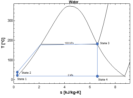
The net work output per unit mass (kJ/kg) and the cycle efficiency. Sketch a T-s diagram for the cycle.
Additional Assumptions:
same assumptions as part (i)
Additional Basic Equations:
None
Solution:
The same analysis from part (i) applies. The only differences are state 1 and 2. Following is the table with known and unknown properties.
| State | T ($^{\circ}$C) | P (kPa) | h (kJ/kg) | s (kJ/kg-K) | Quality |
|---|---|---|---|---|---|
| 1 | 2 | ||||
| 2 | 1000 | 0 | |||
| 3 | 179.88 | 1000 | 2777.1 | 6.5850 | 1 |
| 4 | 17.50 | 2 | 1911.6 | 6.5850 | 0.7474 |
Properties at state 2 can be determined using the SLVM pressure table for the specified pressure ($P_2$) and a quality ($X_2$) of 0. Since the pump process is internally reversible and adiabatic, then the inlet entropy is equal to the outlet entropy ($s_1=s_2$) and state 1 is defined since $P_1$ is also known. State 1 is a two-phase mixture, so that the quality and other properties can be determined from the known value of s_2 and saturation properites. The completed table based on the properties on the ME 200 website is as follows.
| State | T ($^{\circ}$C) | P (kPa) | h (kJ/kg) | s (kJ/kg-K) | Quality |
|---|---|---|---|---|---|
| 1 | 17.50 | 2 | 619.18 | 2.1381 | 0.2219 |
| 2 | 179.88 | 1000 | 762.52 | 2.1381 | 0 |
| 3 | 179.88 | 1000 | 2777.1 | 6.5850 | 1 |
| 4 | 17.50 | 2 | 1911.6 | 6.5850 | 0.7474 |
The computer-generated properties for the new states are as follows.
import CoolProp.CoolProp as CP
import numpy as np
from tabulate import tabulate
h_2 = CP.PropsSI('H','P',P_2*1000,'Q',X_2,'Water')/1000. # enthalpy of water at state 2 [kJ/kg]
s_2 = CP.PropsSI('S','P',P_2*1000,'Q',X_2,'Water')/1000. # entropy of water at state 2 [kJ/kgK]
T_2 = CP.PropsSI('T','P',P_2*1000,'Q',X_2,'Water') # temperature of water at state 2 [K]
s_1 = s_2 # entropy of water at state 1 [kJ/kgK]
h_1 = CP.PropsSI('H','P',P_1*1000,'S',s_1*1000,'Water')/1000. # enthalpy of water at state 1 [kJ/kg]
X_1 = CP.PropsSI('Q','P',P_1*1000,'S',s_1*1000,'Water') # quality of water at state 1
myData = [("1",P_1,T_1-273.15,X_1,h_1,s_1),("2",P_2,T_2-273.15,X_2,h_2,s_2),
("3",P_3,T_3-273.15,X_3,h_3,s_3),("4",P_4,T_4-273.15,X_4,h_4,s_4)]
headers = ["State","P(kPa)","T(C)","X(-)","h(kJ/kg)","s(kJ/kg-K)"]
print(tabulate(myData,headers=headers,tablefmt="fancy_grid",floatfmt=(".0f",".0f","0.1f","0.4f","0.1f","0.5f")))
Updated values of work and heat transfer per unit mass along with cyce efficiency are determined in the following.
w_34 = h_3 - h_4        # turbine work output [kJ/kg]
w_12 = h_1 - h_2        # pump work input [kJ/kg]
q_23 = h_3 - h_2        # boiler heat input [kJ/kg]
w_net = w_34 + w_12     # cycle net work output [kJ/kg]
eta_th = w_net/q_23     # cycle efficiency

print('w_34 = ',round(w_34,1),'kJ\kg')
print('w_12 = ',round(w_12,3),'kJ\kg')
print('q_23 = ',round(q_23,1),'kJ\kg')
print('w_net = ',round(w_net,1),'kJ\kg')
print('eta_th = ',round(eta_th,3))
Since all the processes are internally eversible and the heat transfer processes are isothermal, it is interesting to compare this efficiency with Carnot efficiency operating between a high temperature source of $T_H = T_2$ and $T_C = T_1$.
eta_rev = 1 - T_1/T_2
print('eta_rev',round(eta_rev,3))
Not surprisingly, the efficiencies are the same since all the processes are reversible. This is an improvement over the cycle in part (i). However, it is not practical to build a two-phase pump. Also, the two-phase exit condition for the turbine is problematic.
Part(iii): Rankine Cycle with Imperfect Turbine and Pump
Given:
The same cycle and properties as for part (i), except we'll use isentropic efficiencies of 0.8 for the pump and turbine. We can use the exit states from the pump and turbine as the isentropic states in this problem. All other properties from part (i) can be used.
#Given Inputs:
X_1 = 0. # quality at the pump inlet
eta_p = 0.8 # pump isentropic efficiency
eta_t = 0.8 # turbine isentropic efficiency
Find:
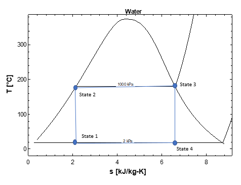
The net work output per unit mas (kJ/kg) and the cycle efficiency. Sketch a T-s diagram for the cycle.
Additional Assumptions:
None: The pump and turbine are no longer internally reversible.
Additional Basic Equations:
$$\eta _p = \dfrac{w_s}{w_{act}}, \eta _t = \dfrac{w_{act}}{w_s}$$Solution:
From part (i), we have the following property table.
| State | T ($^{\circ}$C) | P (kPa) | h (kJ/kg) | s (kJ/kg-K) | Quality |
|---|---|---|---|---|---|
| 1 | 17.50 | 2 | 73.428 | 0.26056 | 0 |
| 2s | 17.50 | 1000 | 74.427 | 0.26056 | - |
| 2 | 1000 | ||||
| 3 | 179.88 | 1000 | 2777.1 | 6.5850 | 1 |
| 4s | 17.50 | 2 | 1911.6 | 6.5850 | 0.7474 |
| 4 | 2 |
Using definitions for isentropic efficiency for a pump and a turbine and simplifying for the assumptions of adiabatic and negligible changes in kinetic and potential energy leads to the following. v
$$\eta_t = \dfrac{w_{act}}{w_s} = \dfrac{h_3-h_4}{h_3-h_{4s}}$$$$\eta_p = \dfrac{W_s}{W_{act}} = \dfrac{h_1-h_{2s}}{h_1-h_2}$$Then, the exit enthalpies are determined as
$$h_4 = h_3 - \eta_t (h_3-h_{4s})$$$$h_2 = h_1 + (h_2s-h_1)/\eta_p$$These enthalpies can be used along with known pressures to determine properties for states 2 and 4. State 2 is a compressed liquid, while state 4 is a superheated vapor. The completed table based on the properties on the ME 200 website is as follows.
| State | T ($^{\circ}$C) | P (kPa) | h (kJ/kg) | s (kJ/kg-K) | Quality |
|---|---|---|---|---|---|
| 1 | 17.50 | 2 | 73.428 | 0.26056 | 0 |
| 2s | 17.50 | 1000 | 74.427 | 0.26056 | - |
| 2 | 17.6 | 1000 | 74.68 | 0.26142 | - |
| 3 | 179.88 | 1000 | 2777.1 | 6.5850 | 1 |
| 4s | 17.50 | 2 | 1911.6 | 6.5850 | 0.7474 |
| 4 | 17.5 | 2 | 2084.7 | 7.1806 | 0.8178 |
The computer-generated properties for the new states are as follows.
import CoolProp.CoolProp as CP
import numpy as np
from tabulate import tabulate
h_1 = CP.PropsSI('H','P',P_1*1000,'Q',X_1,'Water')/1000. # enthalpy of water at state 1 [kJ/kg]
s_1 = CP.PropsSI('S','P',P_1*1000,'Q',X_1,'Water')/1000. # entropy of water at state 1 [kJ/kgK]
T_1 = CP.PropsSI('T','P',P_1*1000,'Q',X_1,'Water') # temperature of water at state 1 [K]
s_2s = s_1 # entropy of water at state 2s [kJ/kgK]
h_2s = CP.PropsSI('H','P',P_2*1000,'S',s_2s*1000,'Water')/1000. # enthalpy of water at state 2s [kJ/kg]
T_2s = CP.PropsSI('T','P',P_2*1000,'S',s_2s*1000,'Water') # temperature of water at state 2s [K]
h_2 = h_1 + (h_2s-h_1)/eta_p # enthalpy of water at state 2 [kJ/kg]
s_2 = CP.PropsSI('S','P',P_2*1000,'H',h_2*1000,'Water')/1000. # entropy of water at state 2 [kJ/kgK]
T_2 = CP.PropsSI('T','P',P_2*1000,'H',h_2*1000,'Water') # temperature of water at state 2 [K]
h_3 = CP.PropsSI('H','P',P_3*1000,'Q',X_3,'Water')/1000. # enthalpy of water at state 3 [kJ/kg]
s_3 = CP.PropsSI('S','P',P_3*1000,'Q',X_3,'Water')/1000. # entropy of water at state 3 [kJ/kgK]
T_3 = CP.PropsSI('T','P',P_3*1000,'Q',X_3,'Water') # temperature of water at state 3 [K]
s_4s = s_3 # entropy of water at state 4s [kJ/kgK]
h_4s = CP.PropsSI('H','P',P_4*1000,'S',s_4s*1000,'Water')/1000. # enthalpy of water at state 4s [kJ/kg]
T_4s = CP.PropsSI('T','P',P_4*1000,'S',s_4s*1000,'Water') # temperature of water at state 4s [K]
X_4s = CP.PropsSI('Q','P',P_4*1000,'S',s_4s*1000,'Water') # quality of water at state 4s [K]
X_4s = round(X_4s,4)
h_4 = h_3 - eta_t*(h_3-h_4s) # enthalpy of water at state 4 [kJ/kg]
s_4 = CP.PropsSI('S','P',P_4*1000,'H',h_4*1000,'Water')/1000. # entropy of water at state 4 [kJ/kgK]
T_4 = CP.PropsSI('T','P',P_4*1000,'H',h_4*1000,'Water') # temperature of water at state 4 [K]
X_4 = CP.PropsSI('Q','P',P_4*1000,'S',s_4*1000,'Water') # quality of water at state 4 [K]
X_4 = round(X_4,4)
myData = [("1",P_1,T_1-273.15,X_1,h_1,s_1),("2s",P_2,T_2s-273.15,"-",h_2s,s_2s),("2",P_2,T_2-273.15,"-",h_2,s_2),
("3",P_3,T_3-273.15,X_3,h_3,s_3),("4s",P_4,T_4s-273.15,X_4s,h_4s,s_4s),("4",P_4,T_4-273.15,X_4,h_4,s_4)]
headers = ["State","P(kPa)","T(C)","X(-)","h(kJ/kg)","s(kJ/kg-K)"]
print(tabulate(myData,headers=headers,tablefmt="fancy_grid",floatfmt=(".0f",".0f","0.1f","0.3f","0.1f","0.5f")))
Finally, this updated data can be used to determine udated values of work and heat transfer per unit mass along with cyce efficiency.
w_34 = h_3 - h_4        # turbine work output [kJ/kg]
w_12 = h_1 - h_2        # pump work input [kJ/kg]
q_23 = h_3 - h_2        # boiler heat input [kJ/kg]
w_net = w_34 + w_12     # cycle net work output [kJ/kg]
eta_th = w_net/q_23     # cycle efficiency

print('w_34 = ',round(w_34,1),'kJ\kg')
print('w_12 = ',round(w_12,3),'kJ\kg')
print('q_23 = ',round(q_23,1),'kJ\kg')
print('w_net = ',round(w_net,1),'kJ\kg')
print('eta_th = ',round(eta_th,3))
The efficiency is significantly lower than for part (i) due to more realistic turbine performance.