Part (i): Geothermal Power Plant
Given:
An engineer working for a large utility company in the west is considering the development of a geothermal power plant. For the site under consideration, this involves drilling a deep well to get access to a high temperature heat source for operating a heat engine. It is assumed that the ground temperature increases with depth with a gradient of 40 °C/km, the heat removal rate from the ground source will be 5 MW, the power plant efficiency will be 50% of the maximum possible efficiency,the above ground temperature is 20 °C, the power plant will continuously generate electricity, the power plant can generate income of 0.08 $/kWh above regular operating costs, and drilling a well to 6 km will cost 5 million dollars more than drilling to 4 km.
# Given Inputs
Delta_Cost = 5e6          # Cost differential for a 6 km well compared to a 4 km well [$]
T_L = 20 + 273.15         # Above ground temperature [K]
Grad_T = 40               # Temperature gradient [°C/km]
Q_dot_H = 5               # Source heat transfer removal rate [MW]
I_elec = 0.08             # Power plant income per unit of electricity delivered [$/kWh]
d_1 = 4                   # First well depth [km]
d_2 = 6                   # Second well depth [km]
Find:
How many years it will take to pay off the additional cost of the 6 km well compared to the 4 km well? Which option would you recommend?
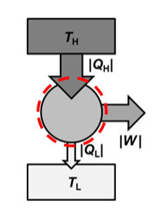
System Sketch:
The heat engine is the system. It receives heat from the underground source and rejects heat to a sink above the ground.
Assumptions:
1) reversible heat engine for maximum possible efficiency, 2) sink and source temperatures are constant
Basic Equations:
$$\eta_{th} = \frac{\dot W_{net,out}}{\dot Q_{H}} = 1 - \frac{\dot Q_{C}}{\dot Q_{H}}$$$$\eta_{th,rev}= 1 - \frac{T_{C}}{T_{H}}$$Solution:
The source temperature is estimated for different depths according to
$$T_{H} = T_L + \nabla T \cdot d$$where $T_L$ is the surface ambient temperature, $\nabla T$ is the gradient, and $d$ is the depth below the surface.
T_H_1 = T_L + d_1*Grad_T   # Source temperature for 4 km well [K]
T_H_2 = T_L + d_2*Grad_T   # Source temperature for 6 km well [K]

print('T_H_1 = ',round(T_H_1,2),'K')
print('T_H_2 = ',round(T_H_2,2),'K')
Next, the maximum possible efficiency for a reversible heat engine is determined for the source temperatures at the two depths. Note that the temperatures must be measured on an absolute scale in order for the result to be valid.
eta_max_1 = 1 - (T_L/T_H_1)          # Reversible heat engine efficiency for 4 km well [-]
eta_max_2 = 1 - (T_L/T_H_2)          # Reversible heat engine efficiency for 6 km well [-]

print('eta_max_1 = ',round(eta_max_1,2))
print('eta_max-2 = ',round(eta_max_2,2))
The actual power plant efficiencies are estimated to be 50% of the maximum possible efficiency for each depth:
$$\eta_{HE} = 0.5 * \eta_{th,rev}$$This efficiency can then be used to calculate the maxmimum power output for each heat engine:
$$\dot W_{net,out} = \eta_{HE} \cdot \dot Q_{H} $$eta_1 = 0.5*eta_max_1 # estimated power plant efficiency for 4 km well [-]
W_dot_1 = eta_1*Q_dot_H # power output from 4 km well [MW]
eta_2 = 0.5*eta_max_2 # estimated efficiency for 6 km well [-]
W_dot_2 = eta_2*Q_dot_H # power output from 6 km well [MW]
print('W_dot_1 = ',round(W_dot_1,3),'MW')
print('W_dot_2 = ',round(W_dot_2,3),'MW')
The more efficient option (6 km) will generate more income each year because of greater power production, but will cost significantly more to install. The payback period ($\Delta t_p$) is determined as the time required for the extra income to equal the extra investment cost.
$$\Delta t_p \cdot \left( \dot W_2 - \dot W_1 \right)I_{elec} = Cost_2 - Cost_1$$Note that power output and rate of income need to be in consistent units. Also, the payback period is expressed in years (8760 hours per year).
Delta_W_dot = W_dot_2 - W_dot_1                    # Additional power output for 6 km well [MW]
Delta_Yr_Income = Delta_W_dot*1000*I_elec*8760.    # Additional yearly income for 6 km well [$]
Delta_t_yr = Delta_Cost/Delta_Yr_Income            # Payback period for 6 km well [yr]

print('Payback period = ',round(Delta_t_yr,1),'years')
Given the very long payback period for the 6 km well, the 4 km well is the better option. This would undoubtedly improve if the heat could be removed at greater rate from the ground leading to higher power production and income.
Part (ii): NASA PV
Given:
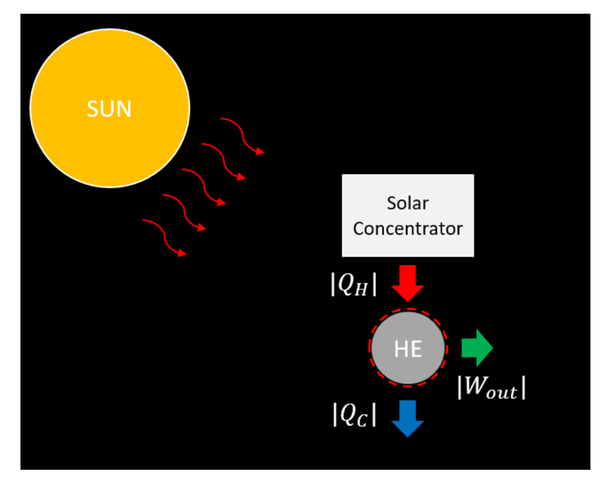
A NASA engineer is considering future replacement of the photovoltaic (PV) solar panels used for the International Space Station. The current panels have a photovoltaic efficiency ($\eta_{PV}$) of about 14% (ratio of electricity produced to incident solar radiation). Two types of replacements are being considered: 1) new high-performance PV panels that have an efficiency ($\eta_{PV}$) of 24% and 2) a Stirling cycle (heat engine) with a heat transfer from concentrating solar collectors (heat source) and a heat transfer to deep space (heat sink). For the Stirling cycle, the engineer has estimated that the solar concentrating collectors provide heat transfer to the cycle at a temperature of 1000 °C by converting 60% of the incident radiation ($\eta_{solar}$ = 0.60). The Stirling cycle also has heat transfer to a deep space temperature of 4 K.
eta_pv = 0.24                   # New photovoltaic efficiency [-]
eta_conc = 0.6                  # Solar conversion efficiency for solar concentrating collector [-]
T_solar = 1000 + 273.15         # Source temperature from solar concentrators[K]
T_space = 4                     # Sink temperature for deep space [K]
Find:
Assuming that the Stirling cycle can achieve an efficiency ($\eta_{Stirling}$) of 50% of the maximum possible efficiency, then determine which of the two options has the highest overall efficiency ($\eta_{total}$ = ratio of electricity produced to incident radiation). Determine the ratio of solar collector area for the worst to the best option. Note that for the PV, $\eta_{total}$ = $\eta_{PV}$, whereas for the Stirling cycle, $\eta_{total}$ = $\eta_{solar}$$\eta_{Stirling}$.
Assumptions:
1) reversible heat engine for maximum possible efficiency, 2) sink and source temperatures are constant
Basic Equations:
$$\eta_{th} = \frac{\dot W_{net,out}}{\dot Q_{H}} = 1 - \frac{\dot Q_{C}}{\dot Q_{H}}$$$$\eta_{th,rev}= 1 - \frac{T_{C}}{T_{H}}$$Solution:
The maximum possible efficiency for a reversible heat engine is determined using source and sink temperatures measured on a absolute temperature scale. For this analysis, the source is the concentrating solar collector that operates at 1000 C (1273 K) and the sink is deep space at 4 K.
$$\eta_{max} = 1 - \dfrac{T_{space}}{T_{solar}}$$The actual stirling efficiency is then estimated to be 50% of this maximum.
eta_th_rev = 1 - (T_space/T_solar)   # Reversible heat exchanger efficiency [-]
eta_Stirling = 0.5*eta_th_rev        # Estimated Stirling engine efficiency [-]

print('eta_th_rev = ',round(eta_th_rev,3))
print('eta_Stirling = ',round(eta_Stirling,3))
The heat source for the Stirling cycle is a solar collector that concentrates solar radiation from the sun and transfers heat to the cycle. Only 60% of the incident (short-wave) solar radiation results in useful heat transfer and the rest (40%) is lost to the surroundings through long-wave radiation. Thus, the overall conversion efficiency for the solar thermal power plant from incident solar radiation to power production is
$$\eta_{SolarThermal} = \eta_{conc} \cdot \eta_{Stirling}$$eta_SolarThermal = eta_conc*eta_Stirling # Overall efficiency for solar powered Stirling engine [-]
print('eta_SolarThermal = ',round(eta_SolarThermal,3))
This efficiency is greater than the PV efficiency. Thus, to produce the same power output, the solar thermal option requires less collector area. The ratio of solar PV area to the concentrator collector area is then:
$$A_{ratio} = \dfrac{A_{PV}}{A_{SolarThermal}} = \dfrac{\eta_{SolarThermal}}{\eta_{PV}}$$A_ratio = eta_SolarThermal/eta_pv # ratio of concentrator collector area to solar PV area
print('A_ratio = ',round(A_ratio,2))