ME 200 – Thermodynamics I – Spring 2020
Homework 18: Cycles
Part (i): Steam power plant
Part (ii): Engine-driven air conditioner
# Given Inputs
P_1 = 40*100            # Pressure at state 1 [kPa]
P_2 = 0.2*100           # Pressure at state 2 [kPa]
P_3 = 0.2*100           # Pressure at state 3 [kPa]
P_4 = 40*100            # Pressure at state 4 [kPa]
P_5 = 1*100             # Pressure at state 5 [kPa]
P_6 = 1*100             # Pressure at state 6 [kPa]

T_1 = 600               # Temperature at state 1 [°C]
T_5 = 15                # Temperature at state 5 [°C]
T_6 = 35                # Temperature at state 6 [°C]

x_2 = 1                 # Quality at state 2 [-]
x_3 = 0                 # Quality at state 3 [-]

w_pump = -1             # specific work input to pump (negative sign) [kJ/kg]
Find:
(a) thermal efficiency, in %,
(b) the mass flow rate of the cooling water, in kg of cooling water per kg of steam, and
(c) sketch the T-v diagram for the steam power cycle.
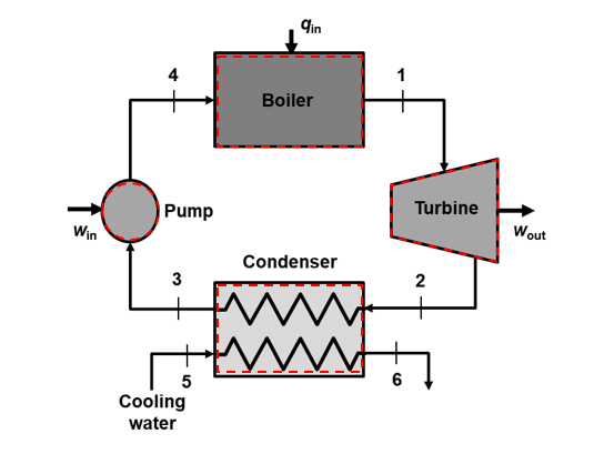
System Sketch:
Each device in the power cycle (pump, boiler, turbine, condenser) is an open system and used to perform mass and energy balances.
Assumptions:
1) steady state, steady flow (SSSF) for all components, 2) neglect changes in pe and ke for each component, 3) neglect heat transfer for pump and turbine
Basic Equations:
$$\dfrac{dE}{dt} = \dot Q- \dot W + \displaystyle\sum_{in} \dot m_{in} (h+ke+pe)_{in}-\displaystyle\sum_{out} \dot m_{out}(h+ke+pe)_{out}$$$$\dfrac{dm}{dt} = \sum \dot m_{in} - \sum \dot m_{out} $$$$\eta_{th} = \dfrac {W_{net,out}} {Q_H}$$$$ h_{comp,liq}(P,T) = h_f(T) + v_f(T) (P - P_{sat}(T))$$or $$dh = cdT + vdP $$
from CoolProp.CoolProp import PropsSI

T_sat_1 = PropsSI('T','P',P_1*1000,'Q',1.0,'Water') - 273.15

print('T_sat_1 = ',round(T_sat_1,2),'°C')
Since the saturation temperature is less than 600°C. the water at state 1 is a superheated vapor. We could then use the superheated water vapor tables (SHV_Tables) to find specific enthalpy and volume at state 1. However, again we'll use software to get these values.
h_1 = PropsSI('H','P',P_1*1000,'T',T_1+273.15,'Water')/1000.
v_1 = 1./PropsSI('D','P',P_1*1000,'T',T_1+273.15,'Water')

print('h_1 = ',round(h_1,1),'kJ/kg')
print('v_1 = ',round(v_1,5),'m^3/kg')
State 2:
State 2 is a saturated vapor ($x_2=1.0$) at a pressure of 20 kPa. Therefore, the temperature and enthalpy are as follows.
T_2 = PropsSI('T','P',P_2*1000,'Q',x_2,'Water') - 273.15
h_2 = PropsSI('H','P',P_2*1000,'Q',x_2,'Water')/1000.

print('T_2 = ',round(T_2,2),'°C')
print('h_2 = ',round(h_2,1),'kJ/kg')
State 3:
State 3 is a saturated liquid ($x_3=1.0$) at a pressure of 20 kPa.
T_3 = PropsSI('T','P',P_3*1000,'Q',x_3,'Water') - 273.15
h_3 = PropsSI('H','P',P_3*1000,'Q',x_3,'Water')/1000.

print('T_3 = ',round(T_3,2),'°C')
print('h_3 = ',round(h_3,1),'kJ/kg')
State 4:
Only the pressure is known for state 4. However, the specific pump work is given and can be used to determine the enthalpy at state 4.
Selecting the pump as the system and appying a mass balance with the steady flow assumption gives:
$$\dot m_{4} = \dot m_{3}$$A steady state energy balance applied to the pump for the given assumptions leads to:
$$0 = 0 - \dot W_{pump} + \dot m_{3} h_{3} - \dot m_{4} h_{4}$$Then, combining the two equations and solving for the enthalpy at state 4 gives:
$$h_4 = h_3 - \dfrac{\dot W_{pump}}{\dot m_3} = h_3 - w_{pump}$$h_4 = h_3 - w_pump # Enthalpy at state 4 [kJ/kg]
print('h_4 = ',round(h_4,1), 'kJ/kg')
We need to check the condition of state 4 by comparing this enthalpy to the saturated liquid and vapor enthalpies at 40 bar.
h_4_f = PropsSI('H','P',P_4*1000,'Q',0.0,'Water')/1000.
h_4_g = PropsSI('H','P',P_4*1000,'Q',1.0,'Water')/1000.

print('h_4_f = ',round(h_4_f,1),'kJ/kg')
print('h_4_g = ',round(h_4_g,1),'kJ/kg')
Since h_4 < h_4_f, it is in compressed liquid state. This makes sense since a pump primarily increases the pressure and has a relatively small impact on temperature. The temperature at state 4 is roughly the same as state 3 due to the nature of the pump and small change of enthalpy. We can determine the temperature by using the incompressible assumption with a constant specific heat for water.
$$h_4 - h_3 = c_w(T_4 - T_3) + v_f(P_4 - P_3)$$or
$$T_4 = T_3 + \dfrac{1}{c_w}(h_4-h_3 - v_f(P_4-P_3))$$c_w = 4.18 # specific heat for liquid water [kJ/kg-K]
v_f = 1./PropsSI('D','T',T_3+273.15,'Q',0.0,'Water') # saturated liquid spec. volume [m^3/kg]
T_4 = T_3 + (h_4 - h_3 - v_f*(P_4-P_3))/c_w # pump leaving temperature (C)
print('T_4 = ',round(T_4,2),'C')
(i): Thermal efficiency
Boiler:
The boiler is an open system with one inlet and one outlet. Under steady flow, $\dot m_1 = \dot m_4$. Then, a steady state energy balance applied to the boiler for the specified set of assumptions can be expressed as
$$0 = \dot Q_{boiler} + \dot m_4 h_4 - \dot m_1 h_1$$which can be rewritten as
$$\dot Q_{boiler} = \dot m_4 (h_1 - h_4)$$or
$$q_{boiler} = \dfrac{\dot Q_{boiler}}{\dot m_4} = h_1 - h_4 $$where $q_{boiler}$ is the heat transfer per unit mass of steam flow.
q_boiler = h_1 - h_4  # Boiler heat input per unit mass of steam flow [kJ/kg]

print('q_boiler = ',round(q_boiler,1), 'kJ/kg')
Turbine:
The turbine is also a single inlet, single outlet open system operating under steady flow ($\dot m_2 = \dot m_1$) and steady state ($dE/dt = 0$) conditions. For the stated assumptions, an energy balance can be simplified to express the work output per unit mass of flow as
$$w_{turbine} = h_1 - h_2 $$w_turbine = h_1 - h_2 # turbine work output per unit mass of flow [kJ/kg]
print('w_turbine = ',round(w_turbine,1), 'kJ/kg')
Overall system efficiency:
The overall effciency can be expressed as the ratio of the net work output per unit mass of flow to the boiler heat transfer per unit mass of flow.
$$\eta_{th} = \dfrac {w_{turbine}+w_{pump}}{q_{boiler}}$$eta_th = (w_turbine + w_pump)/q_boiler # thermal efficiency
print('Thermal Efficiency = ',100*round(eta_th,2),'%')
(ii): Cooling water mass flow rate
Condensor:
If we choose the entire condenser as the system, then the overall energy balance reduces to the following for the specified set of assumnptions.
$$0 = 0 - 0 + \dot m_2 h_2 + \dot m_5 h_5 - \dot m_3 h_3 - \dot m_6 \dot h_6$$For steady flow, $\dot m_3 = \dot m_2 = \dot m_{steam}$ and $\dot m_6 = \dot m_5 = \dot m_{water}$. Then,
$$\dfrac{\dot m_{water}}{\dot m_{steam}} = \dfrac{h_2 - h_3}{h_6 - h_5}$$States 5 and 6 are compressed liquid water since the temperatures are well below the saturation temperature of 100°C at 1 bar. We could estimate the enthalpy for each state using $h_{comp,liq}(P,T) = h_f(T) + v_f(T) (P - P_{sat}(T))$. However, it is more straightforward and sufficiently accurate to assume an incompressible substance with constant specific heat since the temperature change is relativelhy small. Then the enthalpy change of the water is
$$h_6 - h_5 = c_w(T_6 - T_5) + v_f(P_6 - P_5)=c_w(T_6 - T_5)$$since $P_6=P_5$.
c_w = 4.18                             # specific heat for liquid water [kJ/kg-K]
m_ratio = (h_2 - h_3)/c_w/(T_6 - T_5)  # flow rate ratio

print('m_water/m_steam = ',round(m_ratio,1), 'kg/kg')
Property Table for Steam:
| State | P (bar) | T ($^{\circ}$C) | x |
|---|---|---|---|
| 1 | 40 | 600 | - |
| 2 | 0.20 | 60.06 | 1 |
| 3 | 0.20 | 60.06 | 0.00 |
| 4 | 40 | 59.33 | - |
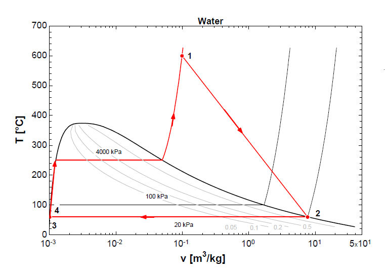
(iii) T-v diagram:
Part(ii): Engine-driven air conditioner
Given:
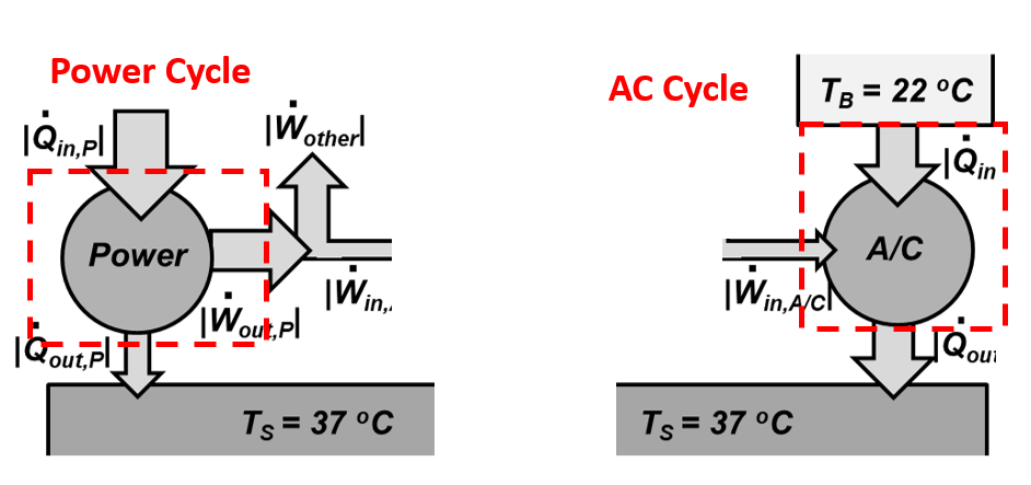
A solar power cycle has a heat input rate of 38 kW. A fraction of the power generated by the power cycle is used to drive an air-conditioning unit that removes heat from a building at a rate of 7 kW and has a COP of 3.5 The power cycle generates an additional 16 kW of power for other purposes.
Notice the sign convention for cycle analysis and the arrow direction across the system boundaries in the sketches below.
# Given Inputs
Q_dot_in_P = 38    # Solar heat transfer rate to the power cycle [kW]
W_dot_other = 16   # Power generated by the power cycle not used for the air conditioner [kW]
Q_dot_in_AC = 7    # Heat transfer to the AC due to cooling the building [kW]
COP_AC = 3.5       # Coefficient of performance of the air-conditioning unit
Find:
(a) Power required for operating the AC in kW
(b) Thermal efficiency in % for power cycle
(c) Total heat transfer rate to the surroundings for both cycles in kW
System Sketch:
We need a system for the AC to determine its power input requirement and heat rejection rate and another system for the power cycle to determine its heat rejection rate to the surroundings.
Assumption:
1) closed system, 2) steady state
Basic Equations:
$$\dfrac{dE}{dt} = \dot Q- \dot W$$$$ COP_R = \dfrac{Q_C}{W_{net_in}}$$$$\eta_{th} = \dfrac {W_{net,out}} {Q_H}$$Solution:
There are two cycles in this problem: a power cycle and an air-conditioing (AC) cycle. Since the cooling load ($\dot Q_{in,AC}$) and the COP are known for the AC cycle, we'll start with this.
a) Power required for AC cycle:
COP for a cooling cycle is defined as the ratio of the cooling rate provided (heat transfer rate to the cycle, $\dot Q_{AC,in}$) to the power input requirement ($\dot W_{in,AC}$). Therefore,
$$\dot W_{in,AC} = \dfrac{\dot Q_{in,AC}}{COP_{AC}}$$Then, the heat rejection rate to the surroundings can be determined from an steady state ($dE/dt=0$) energy balance applied to the AC cycle, which reduces to
$$\dot Q_{net} = \dot W_{net}$$where for this problem: $\dot Q_{net} = \dot Q_{in,AC} - \dot Q_{out,AC}$ and $W_{net} = -\dot W_{in,AC}$.
Note the special sign convention used for cycles where the subscript "in" denotes that energy transfer (heat or work transfer) to the system is positive and "out" denotes that energy transfer (heat or work) from the system is positive. This is a sign convention that is often used for cycle analysis. Then, the heat transfer rate to the surroundings for the air condioning unit is
$$\dot Q_{out,AC} = \dot W_{in,AC} + \dot Q_{in,AC}$$W_dot_in_AC = (Q_dot_in_AC)/COP_AC # Power input required for the AC [kW]
Q_dot_out_AC = W_dot_in_AC + Q_dot_in_AC # Heat transfer to surroundings from AC [kW]
print('W_dot_in_AC = ',round(W_dot_in_AC,2),'kW')
print('Q_dot_out_AC = ',round(Q_dot_out_AC,2),'kW')
b) Thermal efficieny in % for power cycle :
The total power generated is the some of the power input requirement for the AC and power for other purposes that was specified. Then, the overall efficiency of the power cycle is determined as
$$\eta_{th} = \dfrac{\dot W_{in,AC} + \dot W_{other}}{\dot Q_{in,P}}$$W_dot_out_P = W_dot_in_AC + W_dot_other # Total power output for the power cycle[kW]
eta_th = W_dot_out_P/Q_dot_in_P # Thermal efficiency
print('power cycle thermal efficiency = ',round(eta_th*100,1), '%')
c) Total heat transfer to the surroundings:
We already determined the heat transfer to the surroundings for the AC in part a. For the power cycle, the diffference between the heat rate supplied to the cycle and the total power output is the heat transfer rate to surroundings for the power cycle.
$$\dot Q_{out,P} = \dot Q_{in,P} - \dot W_{out,P} $$Q_dot_out_P = Q_dot_in_P - W_dot_out_P # Heat transfer to surroundings from power cycle [kW]
Q_dot_out = Q_dot_out_P + Q_dot_out_AC # Total heat transfer surroundings [kW]
print('Q_dot_out_P = ',round(Q_dot_out_P,2),'kW')
print('Q_dot_out = ',round(Q_dot_out,2),'kW')
Alternative method for part c:
The combination of the two cycles is chosen as a single system.
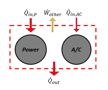
In this case, the power used by the AC is inside the system boundary and the extra power is an output that crosses the system boundary. The heat transfer across the boundary is the solar energy input, the heat input from room to the AC due to cooling, and the overall heat transfer to the surroundings. A steady state energy balance on this system gives
$$ 0 = \dot Q_{net} - \dot W_{net} = \dot Q_{in,P} + \dot Q_{in,AC} - \dot Q_{out} - \dot W_{other} = 0 $$Q_dot_power = 38 # Heat transfer to system from solar [kW]
Q_dot_out_alt = Q_dot_in_P + Q_dot_in_AC - W_dot_other # Heat transfer to surroundings [kW]
print('Q_dot_out_alt = ',round(Q_dot_out_alt ,2),'kW')